Topic 11.1 Notes – Electric Current

1. What Electric Current Is

At its core, electric current is how fast charge flows past a point.

$$I = \frac{dq}{dt}$$

• Units: coulombs per second = amperes (A)
• If 3 C of charge pass through a cross section in 0.5 s, then $I = 6 \text{ A}$.

This definition is completely general. It doesn’t care what material the charge is moving through.

What causes current?

Charges move in response to an electric potential difference (emf, $\varepsilon$).
That potential difference creates an electric field inside the conductor, which pushes the charge carriers.

No potential difference → no electric field → no net current.

Microscopic model of current

Inside a metal:

• $n$ = number of charge carriers per unit volume
• $q$ = charge of each carrier
• $A$ = cross-sectional area
• $v_d$ = average drift velocity

$$I = nqAv_d$$

Here’s the picture to keep in mind:

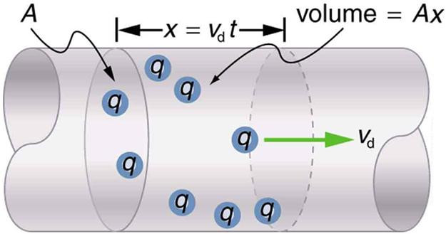
Drift velocity model in a cylindrical conductor

Key ideas:

• Charges move randomly due to thermal motion, but the electric field gives them a small net drift velocity.
• Drift velocity is tiny (often mm/s), but $n$ is huge (~10²⁸ m⁻³ in metals), so current can be large.
• If $v_d = 0$, then $I = 0$, even though individual charges are still moving randomly.

This “random motion + small drift” idea shows up in explanations on FRQs, so say it clearly if asked.

2. Direction of Current

Current has a direction, but it is not a true vector.

• It does not have x- and y-components.
• It does not follow vector addition rules.
• It is a scalar with an assigned direction.

Conventional current vs. electron flow

By definition:

• Conventional current points in the direction positive charge would move.
• In metal wires, the actual charge carriers are electrons (negative).

So:

• Conventional current: from + terminal to − terminal.
• Electron flow: from − terminal to + terminal.

On AP problems, use conventional current unless told otherwise. If you ever compute $nqv_d$ for electrons, remember $q = -e$, so the direction of $\vec{J}$ flips relative to $\vec{v}_d$.

That sign issue is a classic place to lose points.

3. Current Density

When we zoom in further, we talk about current per unit area.

Definition

$$J = \frac{I}{A}$$

Units: A/m²

If 4 A passes uniformly through a 2 m² area, then $J = 2 \text{ A/m}^2$.

Microscopic form

$$\vec{J} = nq\vec{v}_d$$

Important differences from current:

• Current density is a vector.
• It points in the direction of charge flow.
• Its magnitude depends on $n$, $q$, and $v_d$.

If the wire is uniform and the current spreads evenly, $J$ is constant across the cross section. In non-uniform situations, $J$ can vary with position.

Connection to electric field

Inside a conductor:

$$\vec{E} = \rho \vec{J}$$

• $\rho$ = resistivity (material property)
• This is the microscopic form of Ohm’s law.

Interpret it physically:

• Larger $\rho$ → you need a larger electric field to push the same current density.
• Larger $J$ → stronger internal electric field.

This relationship often gets used when deriving macroscopic Ohm’s law $V = IR$.

4. Total Current from Current Density

If current density varies across the cross section, you add up contributions from each tiny area element:

$$I = \int \vec{J} \cdot d\vec{A}$$

Only the component of $\vec{J}$ perpendicular to the surface contributes.

In the cylindrical conductor shown below, the shaded slice represents a cross-sectional area $A$. The total current through that slice is found by integrating $\vec{J}$ over the entire area.

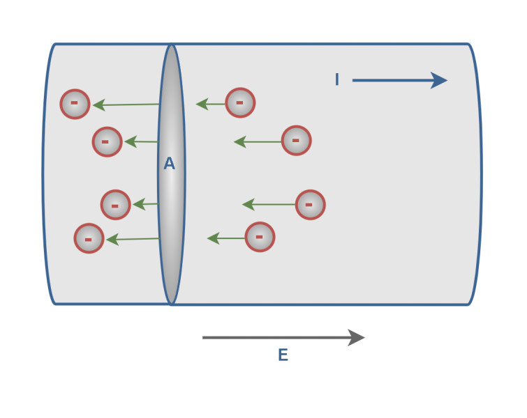
Current through a cross section of a cylindrical conductor

How this plays out on problems:

1. Identify how $\vec{J}$ depends on position.
2. Write $dA$ (often $2\pi r\,dr$ for circular symmetry).
3. Compute $\vec{J} \cdot d\vec{A}$.
4. Integrate over the entire area.

If $\vec{J}$ is uniform and perpendicular to the surface, it simplifies to:

$$I = JA$$

This integral form connects the microscopic field picture to the measurable current in a circuit.