Topic 8.5 Notes – Electric Flux

1. What Electric Flux Is

When we say flux, we mean “how much of something passes through a surface.” For electric flux, that “something” is the electric field.

So electric flux tells you how much of the electric field crosses a given area. It does not tell you the field at a point. It combines:

• The magnitude of $\vec{E}$
• The size of the surface
• The orientation of that surface

Symbol: $\Phi_E$
Units: $\text{N}\cdot\text{m}^2/\text{C}$ (equivalently $\text{V}\cdot\text{m}$)

Picture field lines crossing a surface:

• More lines crossing → larger flux
• Lines grazing along the surface → little or no flux
• Lines leaving vs. entering → sign matters

Flux can be defined for:

• Open surfaces (a flat sheet, curved patch)
• Closed surfaces (a sphere, cube, any sealed boundary)

For a closed surface, flux represents the net outward field flow through the entire boundary.

2. The Area Vector and the Dot Product

Electric flux is defined using a dot product. That’s where direction enters the picture.

a. The Area Vector

Every surface has an associated area vector $\vec{A}$.

• Magnitude = area of the surface
• Direction = perpendicular (normal) to the surface
• For a closed surface, it always points outward (by convention)
• For an open surface, you choose the direction, but must stay consistent

Here’s what that looks like for a flat surface in a uniform field:

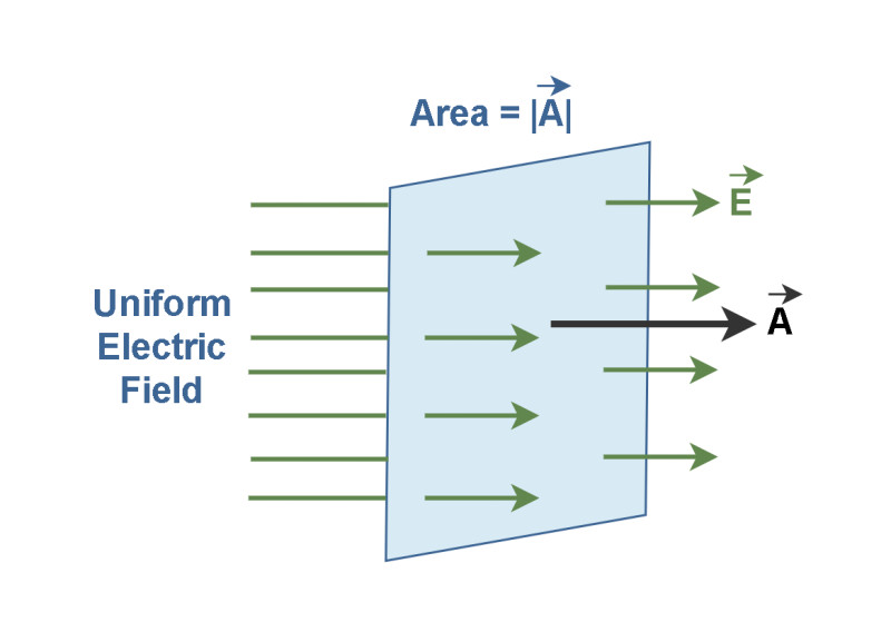
In the diagram, the black arrow labeled $\vec{A}$ is perpendicular to the surface. That perpendicular direction is what determines the sign of flux.

b. Flux in a Constant Electric Field

If the electric field is uniform over a flat surface, flux is:

$$\Phi_E = \vec{E} \cdot \vec{A}$$

Using the dot product definition:

$$\Phi_E = EA\cos\theta$$

where
- $\theta$ is the angle between $\vec{E}$ and $\vec{A}$
- $A$ is the area

The cosine handles both magnitude and sign.

Key cases to recognize instantly:

• Surface perpendicular to field → $\theta = 0^\circ$, flux = $EA$ (maximum)
• Surface tilted → reduced by $\cos\theta$
• Surface parallel to field → $\theta = 90^\circ$, flux = 0

Notice something important: flux depends only on the component of $\vec{E}$ normal to the surface. The parallel component does nothing.

Quick example:
A $2\,\text{m}^2$ surface in a $150\,\text{N/C}$ field at $60^\circ$ to the normal:

$$\Phi_E = (150)(2)\cos 60^\circ = 300(0.5) = 150\,\text{N}\cdot\text{m}^2/\text{C}$$

On multiple choice, they love giving the angle with the surface instead of the normal. If they say the field makes $30^\circ$ with the surface, that means $60^\circ$ with the normal.

3. Electric Flux Through Curved or Nonuniform Surfaces

When $\vec{E}$ varies across the surface or the surface is curved, we use the surface integral:

$$\Phi_E = \int \vec{E} \cdot d\vec{A}$$

Here:

• $d\vec{A}$ is a tiny area patch with its own outward normal
• At each point, $d\Phi = \vec{E} \cdot d\vec{A}$
• The integral adds up all contributions

This definition works for:

• Curved surfaces like spheres or cylinders
• Nonuniform fields
• Closed surfaces

A powerful shortcut idea:

• If $\vec{E}$ is parallel to the surface, then $\vec{E} \cdot d\vec{A} = 0$ there.
• That entire portion contributes zero flux.

Example insight:
If a flat surface lies in the $xy$-plane, its area vector points in the $z$-direction. Any electric field with only $x$ and $y$ components produces zero flux through that surface. This shows up often in free response setups.

4. Flux Through Closed Surfaces

For a closed surface, we write:

$$\Phi_E = \oint \vec{E} \cdot d\vec{A}$$

The circle on the integral reminds you it’s a closed boundary.

Key conventions:

• Area vectors point outward
• Field lines leaving → positive contribution
• Field lines entering → negative contribution

What flux measures here is the net outward flow through the boundary. It does not depend on how complicated the field looks inside.

Important conceptual cases:

• Equal field entering and leaving → net flux = 0
• A strong field does not guarantee large flux if it’s mostly tangent to the surface
• A surface can have nonzero field everywhere and still have zero net flux

This definition is the foundation for Gauss’s law, which connects flux through a closed surface to the charge enclosed.