Topic 9.2 Notes – Electric Potential

1. What Electric Potential Is

Definition

Electric potential $V$ is electric potential energy per unit charge:

$$V = \frac{U_E}{q}$$

• Units: volts (V) where $1\text{ V} = 1\text{ J/C}$
• It is a scalar, so no direction.

If a positive test charge has potential energy $U_E$ at a point, dividing by its charge gives the potential of that location.

Reference Point

For isolated charge distributions, we define
$$V = 0 \quad \text{at infinity}$$

Physically, $V$ tells you the work per unit charge required to bring a positive test charge from infinity to that point.

If it takes positive work to bring it in, the potential there is positive.

Potential Difference

Between two points:

$$\Delta V = \frac{\Delta U_E}{q} \qquad\text{and}\qquad \Delta U_E = q \Delta V$$

Important sign ideas:

• For positive charges: higher $V$ → higher $U_E$.
• For negative charges: energy changes opposite the sign of $\Delta V$.

In circuits, batteries maintain a potential difference by using chemical reactions to separate charge. That separation creates electric potential energy.

2. Electric Potential from Charges

Point Charges

For a single point charge:

$$V = \frac{1}{4\pi\varepsilon_0}\frac{q}{r}$$

• Depends only on distance $r$.
• The sign of $V$ matches the sign of $q$.

If you double the charge, you double the potential. If you double the distance, potential is cut in half.

For multiple point charges:

$$V_{\text{total}} = \sum_i \frac{1}{4\pi\varepsilon_0}\frac{q_i}{r_i}$$

This is scalar superposition. You just add the values algebraically. No components. This is why potential problems are often easier than field problems.

Continuous Charge Distributions

When charge is spread out:

$$V = \frac{1}{4\pi\varepsilon_0}\int \frac{dq}{r}$$

General setup:

1. Choose coordinates.
2. Replace $dq$ with density:
   • $dq = \lambda\,dl$
   • $dq = \sigma\,dA$
   • $dq = \rho\,dV$
3. Express $r$ to the field point.
4. Integrate over the distribution.

On the AP exam, calculus setups are limited to specific geometries:

• Infinitely long wire or cylinder at distance $r$
• Thin ring along its axis
• Semicircular arc at its center
• Finite line charge
  • On its axis
  • On its perpendicular bisector

If you see something outside this list, it’s likely conceptual only.

3. Relationship Between Electric Potential and Electric Field

These two are tightly connected.

Field from Potential

$$\vec{E} = -\nabla V$$

Component form:

$$E_x = -\frac{\partial V}{\partial x}, \quad E_y = -\frac{\partial V}{\partial y}, \quad E_z = -\frac{\partial V}{\partial z}$$

The field points in the direction of steepest decrease in potential.

If $V(x) = 5x^2$, then
$$E_x = -10x$$
The derivative tells you how fast potential changes in space.

On FRQs, they often give you $V(x,y)$ and expect clean partial derivatives.

Potential from Field

$$\Delta V = V_b - V_a = -\int_a^b \vec{E} \cdot d\vec{r}$$

Key pieces:

• Dot product → only the component of $\vec{E}$ along the path matters.
• Negative sign → field points toward decreasing potential.
• Result is path independent because electrostatic fields are conservative.

If you move with the field, potential drops.
If you move against the field, potential increases.

4. Equipotential Lines and Field Maps

Here’s how potential looks in space. For a single positive point charge, the electric field lines radiate outward and the equipotential lines form concentric circles around the charge.

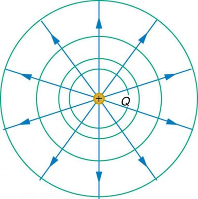
Field lines and equipotentials for a positive point charge

Equipotential Lines

Equipotential lines (or surfaces in 3D) connect points of equal $V$.

Moving along one:

• $\Delta V = 0$
• No work is done by the electric force.

Relationship to the Electric Field

• Equipotentials are perpendicular to electric field vectors.
• Field vectors point toward lower potential.
• Closer spacing of equipotentials → stronger field.
• There is no component of $\vec{E}$ along an equipotential.

In the diagram, notice how each field line crosses the circular equipotentials at right angles. If you’re given one map, you should be able to sketch the other. That shows up in both multiple choice and FRQs.