Topic 13.2 Notes – Electromagnetic Induction

1. What Electromagnetic Induction Is

Electromagnetic induction is the production of an emf (electric potential difference) due to a changing magnetic flux.

Magnetic flux measures how much magnetic field passes through a surface:

$$\Phi_B = \int \vec{B} \cdot d\vec{A}$$

For a flat loop in a uniform field:

$$\Phi_B = BA\cos\theta$$

• $A$ is the area of the loop
• $\theta$ is the angle between B and the area vector (normal to the surface)
• $B\cos\theta$ is the perpendicular component

Here’s what that geometry looks like for a tilted loop in a uniform magnetic field:

The blue arrows represent a uniform $\vec{B}$, and the red vector is the area vector perpendicular to the surface of the loop. The angle $\theta$ between them determines how much of the field actually passes through the loop.

Flux changes if:

• The field strength $B$ changes
• The area $A$ changes
• The orientation $\theta$ changes
• The loop moves into or out of a field region

Faraday’s Law ties flux change to induced emf:

$$\mathcal{E} = -\frac{d\Phi_B}{dt}$$

For $N$ turns:

$$\mathcal{E}_{\text{total}} = -N\frac{d\Phi_B}{dt}$$

That negative sign is Lenz’s law. It tells you the direction.

2. Faraday’s Law in Common Situations

On tests, flux almost always changes in one of these specific ways.

a. Changing Magnetic Field (Area Constant)

If the loop is stationary and only $B$ changes:

$$\mathcal{E} = -A \frac{dB_\perp}{dt}$$

where $B_\perp = B\cos\theta$.

• Bigger loop → bigger emf
• Faster change in $B$ → bigger emf

If a graph of $B$ vs. time is given, the slope gives you $dB/dt$. Students often miss that the rate matters, not the value of $B$.

b. Changing Area (Field Constant)

If $B$ is constant but area changes:

$$\mathcal{E} = -B \frac{dA_\perp}{dt}$$

Classic case: a rectangular loop entering a uniform field at speed $v$.

If one side of length $L$ is cutting into the field:

$$\frac{dA}{dt} = L v$$

So

$$\mathcal{E} = -BLv$$

This is the motional emf result you’ve seen before.

c. Changing Orientation (Rotating Loop)

If the loop rotates with angular speed $\omega$:

$$\Phi_B = BA\cos(\omega t)$$

Then

$$\mathcal{E} = NBA\omega \sin(\omega t)$$

This sinusoidal emf is the basis of AC generators. Maximum emf occurs when flux is changing fastest, not when flux is largest.

d. Solenoids and Multiple Loops

Each loop gets the same induced emf. The total is multiplied by $N$.

More turns → proportionally larger emf.
Nothing fancy. Just multiply.

3. Lenz’s Law and Direction of Induced Current

Lenz’s Law: The induced current creates a magnetic field that opposes the change in flux.

Students lose points here by opposing the field itself. It’s the change that matters.

How to apply it

1. Decide if flux is increasing or decreasing.
2. Figure out what magnetic field would oppose that change.
3. Use the right-hand rule to get current direction.

Right-hand rule:

• Thumb → induced magnetic field
• Curled fingers → current direction

Example patterns:

• Field into page increasing → induced field out of page.
• Field into page decreasing → induced field into page.

If resistance is known:

$$I = \frac{\mathcal{E}}{R}$$

Here’s a standard Lenz’s law setup to picture. The external magnetic field (red dots, out of the page) changes with time. The loop responds by creating its own magnetic field that opposes that change, which sets the direction of the induced current.

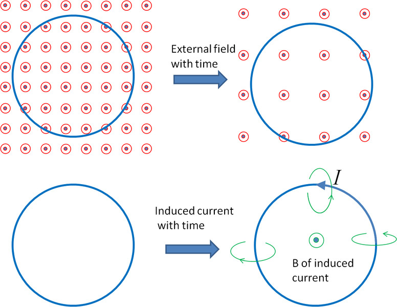
Lenz’s law for a decreasing outward magnetic field

4. Induced Current, Magnetic Force, and Motion

Once current exists, it feels a magnetic force:

$$\vec{F}_B = I \vec{L} \times \vec{B}$$

If perpendicular:

$$F = ILB$$

Important details:

• Only wire segments inside the field feel force.
• The force direction follows current × B.
• The force always opposes the motion that caused the flux change.

Since motional emf often depends on velocity, you get:

$$F \propto v$$

That creates magnetic damping. Plug it into Newton’s second law:

$$F_{\text{net}} = ma$$

This shows up on FRQs where acceleration decreases as velocity increases.

5. Faraday’s Law in Maxwell’s Equations and EM Waves

Maxwell’s third equation (integral form) is:

$$\oint \vec{E} \cdot d\vec{l} = -\frac{d\Phi_B}{dt}$$

This says a changing magnetic field creates a circulating electric field, even without wires.

That electric field can then change in time and create a magnetic field. The coupling of changing electric and magnetic fields produces electromagnetic waves that travel at speed $c$ in free space.

You are not expected to derive $c$. Just understand that induction is part of the full electromagnetic framework.