Topic 2.3 Notes – Price Elasticity of Demand
1. What Price Elasticity of Demand Is
Price Elasticity of Demand (PED) measures how responsive quantity demanded is to a change in a good’s own price.
Economists use elasticity to measure percentage changes in quantity caused by changes in:
- Own price (this topic)
- Income
- Prices of related goods (substitutes and complements)
For this unit, we focus on own-price elasticity.
The Formula
- It’s a percentage over percentage comparison.
- Because of the Law of Demand, is usually negative.
- On the AP exam, we almost always use the absolute value.
Midpoint Formula
When calculating between two points, use the midpoint method so your answer doesn’t change depending on direction:
Quick example:
Price rises from 20 to 24. Quantity falls from 50 to 40.
Absolute value 1.22 → elastic.
Slope Is Not Elasticity
- Slope = change in Q over change in P.
- Elasticity = % change in Q over % change in P.
On a linear demand curve, slope is constant. Elasticity is not. That difference shows up constantly on MCQs.
2. The Five Types of Elasticity
The benchmark number is 1.
Perfectly Inelastic (Ed = 0)
- Quantity does not change at all.
- Vertical demand curve.
- Example: life-saving insulin in extreme cases.
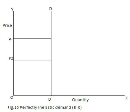
Perfectly inelastic demand (vertical curve, Ed = 0)
Relatively Inelastic (0 < Ed < 1)
- %ΔQ < %ΔP.
- Steep demand curve.
- Examples: gasoline in the short run, cigarettes.
Unit Elastic (Ed = 1)
- %ΔQ = %ΔP.
- Total revenue stays constant when price changes.
- Occurs at the midpoint of a linear demand curve.
Relatively Elastic (Ed > 1)
- %ΔQ > %ΔP.
- Flatter demand curve.
- Examples: restaurant meals, vacations, luxury goods.
Perfectly Elastic (Ed = ∞)
- Consumers buy only at one price.
- Horizontal demand curve.
- Seen in the perfectly competitive firm model where the firm is a price taker.
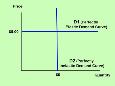
Perfectly elastic (horizontal) and perfectly inelastic (vertical) demand
Perfectly elastic and perfectly inelastic are theoretical extremes. They help you think clearly about responsiveness.
3. Elasticity Along a Demand Curve
On a straight-line demand curve, elasticity changes as you move from top to bottom:
- Top (high P, low Q) → Elastic
- Middle → Unit elastic
- Bottom (low P, high Q) → Inelastic
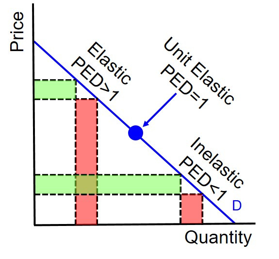
Elasticity along a straight-line demand curve
Why this happens:
At high prices and low quantities, a given dollar change is a small percentage of price but causes a large percentage change in quantity. At low prices and high quantities, that same dollar change is a large percentage of price but small relative to quantity.
Always think in percentages.
4. The Total Revenue Test
Total Revenue is:
The effect of a price change depends on elasticity.
| Demand Type | Price ↑ | Price ↓ | Why |
|---|---|---|---|
| Elastic (Ed > 1) | TR ↓ | TR ↑ | Quantity changes more than price |
| Inelastic (Ed < 1) | TR ↑ | TR ↓ | Price change dominates |
| Unit Elastic (Ed = 1) | TR unchanged | TR unchanged | Proportional change |
Real-world anchors:
- Cigarette taxes raise government revenue because demand is relatively inelastic.
- Gasoline price spikes increase revenue in the short run for the same reason.
- Airlines lower prices during off-peak times because leisure travel is more elastic.
Firms use this logic constantly when deciding pricing strategies.
5. What Determines Price Elasticity of Demand
Availability of Substitutes
More substitutes → more elastic.
Few substitutes → more inelastic.
Coke has many substitutes. Insulin does not.
Necessities vs. Luxuries
Necessities → inelastic.
Luxuries → elastic.
Proportion of Income
Small share of income → inelastic (salt).
Large share → elastic (cars, tuition).
Time Horizon
More time → more elastic.
Gasoline demand is inelastic in the short run. Over time, people buy fuel-efficient cars or move closer to work, making demand more elastic.
Key Takeaways
Elastic, Inelastic, and Unit Elastic Demand
Greater than 1 is elastic, less than 1 is inelastic, and equal to 1 is unit elastic.
Perfectly Elastic and Perfectly Inelastic Demand
Infinite means quantity changes completely at one price; zero means quantity does not change with price.
Absolute Value of Elasticity
Economists usually ignore the negative sign and compare responsiveness using the coefficient's magnitude.
Elasticity Versus Slope
Responsiveness is based on percentage changes, so it varies along a linear curve even when slope is constant.
Elasticity Along a Linear Demand Curve
It is more elastic at high prices and low quantities, and more inelastic at low prices and high quantities.
Total Revenue
The money a firm receives from sales, calculated as price times quantity sold.
Determinants of Price Elasticity of Demand
Responsiveness depends on factors like substitute availability, necessity, budget share, and time to adjust.
Price Elasticity of Demand
The percent change in quantity demanded divided by the percent change in price.
Total Revenue Test
Price and total revenue move opposite for elastic, together for inelastic, and not at all for unit elastic demand.
Midpoint Formula
A method using average price and quantity to calculate percent changes symmetrically.
Notes
Elastic, Inelastic, and Unit Elastic Demand
Greater than 1 is elastic, less than 1 is inelastic, and equal to 1 is unit elastic.
Perfectly Elastic and Perfectly Inelastic Demand
Infinite means quantity changes completely at one price; zero means quantity does not change with price.
Absolute Value of Elasticity
Economists usually ignore the negative sign and compare responsiveness using the coefficient's magnitude.
Elasticity Versus Slope
Responsiveness is based on percentage changes, so it varies along a linear curve even when slope is constant.
Elasticity Along a Linear Demand Curve
It is more elastic at high prices and low quantities, and more inelastic at low prices and high quantities.
Total Revenue
The money a firm receives from sales, calculated as price times quantity sold.
Determinants of Price Elasticity of Demand
Responsiveness depends on factors like substitute availability, necessity, budget share, and time to adjust.
Price Elasticity of Demand
The percent change in quantity demanded divided by the percent change in price.
Total Revenue Test
Price and total revenue move opposite for elastic, together for inelastic, and not at all for unit elastic demand.
Midpoint Formula
A method using average price and quantity to calculate percent changes symmetrically.
