Topic 3.7 Notes – Perfect Competition
1. What a Perfectly Competitive Market Is
Perfect competition has a very specific structure. That structure forces firms to be price takers and leads to efficiency.
Core characteristics
- Many small firms
Each firm produces a tiny share of total output. No single firm can affect market price. - Identical products
Goods are perfectly standardized. Classic example is agriculture like wheat or corn. One farmer’s wheat is indistinguishable from another’s. - No barriers to entry or exit
Firms can enter when profits exist and leave when losses occur. No patents, high startup costs, or legal restrictions keeping others out. - Perfect information
Buyers and sellers know the market price. - No market power
Because products are identical and there are many firms, no firm can charge above the market price.
This structure creates price takers.
- The market (industry supply and demand) determines price.
- Each firm faces a perfectly elastic (horizontal) demand curve at that price.
- For the firm:
Here’s the classic side-by-side setup. Focus on how the left panel determines the market price, and how that same price appears as a horizontal line for the individual firm on the right.
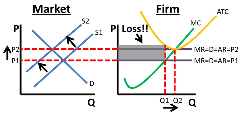
On the left, the intersection of industry supply and demand sets the market price. On the right, the firm takes that price as given, which is why its demand and marginal revenue curves are horizontal.
2. How a Perfectly Competitive Firm Maximizes Profit
Firms maximize economic profit, which equals:
The decision rule is always:
- Produce where MR = MC
- In perfect competition, MR = P
- So produce where P = MC
After finding that quantity, compare P to ATC to see profit or loss.
Short-Run Outcomes
| Situation | Condition at MR = MC | Result |
|---|---|---|
| Short-run profit | Profit rectangle above ATC | |
| Short-run loss (operate) | Loss, but covers variable costs | |
| Shutdown | Produce |
The shutdown rule is huge on tests:
Produce only if .
Why? Because variable costs must be covered in the short run. Fixed costs are sunk.
On FRQs, if they give you numbers, plug them in. For example:
If , , and :
Draw the rectangle between P and ATC at the profit-maximizing quantity.
3. From Short Run to Long Run Equilibrium
The adjustment mechanism is entry and exit.
If firms earn short-run profits
- New firms enter (no barriers).
- Market supply shifts right.
- Market price falls.
- Each firm’s horizontal price line drops.
- Profits shrink to zero.
If firms earn short-run losses
- Firms exit.
- Market supply shifts left.
- Market price rises.
- Remaining firms’ price line rises.
- Losses disappear.
In long-run equilibrium:
- Economic profit = 0 (normal profit only)
- Firms produce at efficient scale
This is the break-even outcome caused by free entry and exit.
4. Why Perfect Competition Is Efficient
Perfect competition achieves both types of efficiency.
Allocative efficiency
- Occurs where .
- Price reflects:
- Marginal benefit (what consumers are willing to pay)
- Marginal cost (cost of the last unit produced)
Resources go to their highest-valued use. No deadweight loss.
Productive efficiency
- Occurs where firms produce at minimum ATC.
- Firms use the least-cost combination of inputs.
In long-run equilibrium:
That’s why this model is the efficiency benchmark when comparing to monopoly or oligopoly.
5. Constant, Increasing, and Decreasing Cost Industries
Long-run price depends on how input costs change as firms enter.
1. Constant Cost Industry
- Entry does not change input prices.
- Long-run price stays the same.
- Long-run supply is perfectly elastic (horizontal).
2. Increasing Cost Industry
- Entry increases input prices (scarce resources).
- Long-run price rises.
- Long-run supply is upward sloping.
3. Decreasing Cost Industry
- Entry lowers input costs (economies of scale, better infrastructure).
- Long-run price falls.
- Long-run supply is downward sloping.
On exams, constant cost is most common. Show the sequence clearly: demand shift → short-run profit/loss → entry/exit → new long-run equilibrium.
Key Takeaways
Perfect Competition
A market with many small firms, identical products, free entry and exit, and no price control.
Price Taker
A firm that must accept the market price because its own output is too small to affect price.
Profit-Maximizing Rule in Perfect Competition
Produce the quantity where marginal cost equals marginal revenue, as long as price covers average variable cost.
Side-by-Side Graphs in Perfect Competition
A market supply-demand graph paired with a firm cost-revenue graph linked by the market price.
Short-Run Profit, Loss, and Shutdown
Profit if price exceeds ATC, loss if AVC < price < ATC, shutdown if price falls below AVC.
Shutdown Point
The minimum average variable cost; below this price, a firm produces zero in the short run.
Economic Profit in Perfect Competition
Total revenue minus total cost; on a graph, it is (price minus ATC) times quantity.
Short-Run Competitive Equilibrium
A temporary market outcome where firms may earn profits, losses, or break even at the current price.
Entry and Exit in Perfect Competition
Profits attract new firms and losses cause firms to leave, shifting market supply.
Efficient Scale
The output level where average total cost is minimized.
Demand Shock in a Perfectly Competitive Market
A demand shift changes market price, creates short-run profit or loss, then triggers entry or exit.
Constant-Cost, Increasing-Cost, and Decreasing-Cost Industries
Industry expansion leaves long-run price unchanged, raises it, or lowers it depending on input cost changes.
Price as a Signal in Perfect Competition
Market price communicates marginal benefits and marginal costs, guiding consumers and producers to efficient choices.
Competitive Firm Demand, Price, and Marginal Revenue
A competitive firm's demand curve is horizontal, so price equals marginal revenue for every unit sold.
Long-Run Competitive Equilibrium and Normal Profit
A market state where firms earn zero economic profit, so no firms enter or exit.
Allocative and Productive Efficiency in Perfect Competition
In long-run equilibrium, price equals marginal cost and minimum average total cost.
Economic Loss in Perfect Competition
Total cost exceeds total revenue; on a graph, it is (ATC minus price) times quantity.
Notes
Perfect Competition
A market with many small firms, identical products, free entry and exit, and no price control.
Price Taker
A firm that must accept the market price because its own output is too small to affect price.
Profit-Maximizing Rule in Perfect Competition
Produce the quantity where marginal cost equals marginal revenue, as long as price covers average variable cost.
Side-by-Side Graphs in Perfect Competition
A market supply-demand graph paired with a firm cost-revenue graph linked by the market price.
Short-Run Profit, Loss, and Shutdown
Profit if price exceeds ATC, loss if AVC < price < ATC, shutdown if price falls below AVC.
Shutdown Point
The minimum average variable cost; below this price, a firm produces zero in the short run.
Economic Profit in Perfect Competition
Total revenue minus total cost; on a graph, it is (price minus ATC) times quantity.
Short-Run Competitive Equilibrium
A temporary market outcome where firms may earn profits, losses, or break even at the current price.
Entry and Exit in Perfect Competition
Profits attract new firms and losses cause firms to leave, shifting market supply.
Efficient Scale
The output level where average total cost is minimized.
Demand Shock in a Perfectly Competitive Market
A demand shift changes market price, creates short-run profit or loss, then triggers entry or exit.
Constant-Cost, Increasing-Cost, and Decreasing-Cost Industries
Industry expansion leaves long-run price unchanged, raises it, or lowers it depending on input cost changes.
Price as a Signal in Perfect Competition
Market price communicates marginal benefits and marginal costs, guiding consumers and producers to efficient choices.
Competitive Firm Demand, Price, and Marginal Revenue
A competitive firm's demand curve is horizontal, so price equals marginal revenue for every unit sold.
Long-Run Competitive Equilibrium and Normal Profit
A market state where firms earn zero economic profit, so no firms enter or exit.
Allocative and Productive Efficiency in Perfect Competition
In long-run equilibrium, price equals marginal cost and minimum average total cost.
Economic Loss in Perfect Competition
Total cost exceeds total revenue; on a graph, it is (ATC minus price) times quantity.
