Topic 6.2 Notes – Externalities

1. What Externalities Are

An externality is a third-party side effect of production or consumption that is not reflected in the market price.

When you buy or sell something, you consider your own costs and benefits. If your decision also affects others who aren’t part of the transaction, that’s an externality.

Externalities usually arise because:

• Property rights aren’t well-defined (no one “owns” clean air).
• Transaction costs are high (too hard for everyone affected to negotiate).

Private vs Social Margins

You already know firms and consumers think at the margin. Now we separate private and social margins.

• MPC (Marginal Private Cost) = cost to producers (the supply curve)
• MSC (Marginal Social Cost) = MPC + external cost
• MPB (Marginal Private Benefit) = benefit to consumers (the demand curve)
• MSB (Marginal Social Benefit) = MPB + external benefit

In a free market:
$$\text{MPB} = \text{MPC}$$

That gives the market equilibrium.

But the socially optimal quantity occurs where:
$$\text{MSB} = \text{MSC}$$

That’s the output that maximizes total economic surplus.

Here’s the key idea you’ll use all year: rational agents respond to private costs and benefits, not external ones. That’s why markets can fail.

2. Negative Externalities and Overproduction

A negative externality creates external costs.

Classic examples:

• Factory pollution contaminating air or water
• Cigarettes and secondhand smoke
• Carbon emissions contributing to climate change

Arthur Pigou first formalized the solution in The Economics of Welfare (1920). That’s where the idea of Pigouvian taxes comes from.

Graphing a Negative Externality

Look at the graph below as the standard model of a negative production externality.

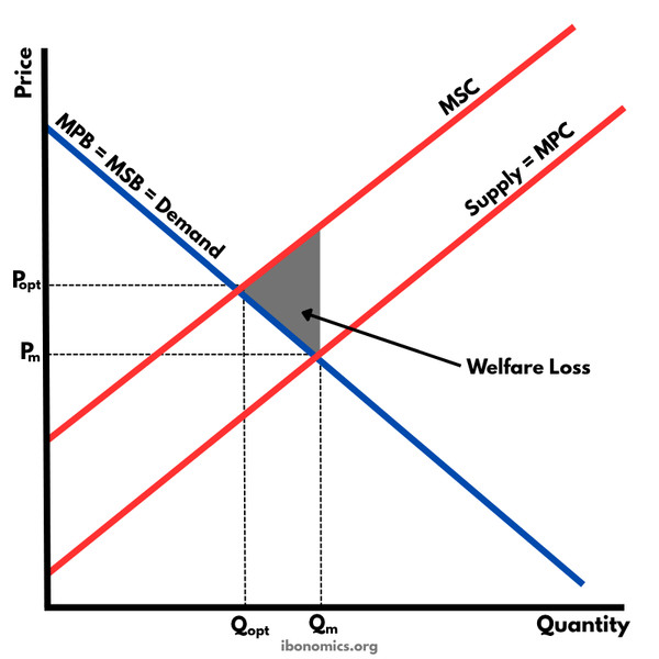
Negative externality of production

On the graph:

• Demand is labeled MPB = MSB (assuming no external consumption benefit)
• Supply is labeled MPC
• The MSC curve lies above MPC (the vertical gap is the marginal external cost)

Free market outcome:

• Where MPB = MPC (labeled $Q_m$ on the graph)
• Quantity is too high
• This is overproduction

Socially optimal outcome:

• Where MSB = MSC (labeled $Q_{opt}$)
• Lower quantity
• Deadweight loss is the shaded triangle between MSC and demand over the extra units from $Q_{opt}$ to $Q_m$.

Important exam move:
The tax size equals the vertical distance between MSC and MPC at the socially optimal quantity.

The tax shifts MPC upward until it equals MSC. Examples include carbon taxes and cigarette taxes.

3. Positive Externalities and Underproduction

A positive externality creates external benefits.

Common examples:

• Vaccinations (herd immunity)
• Education (higher productivity, lower crime)
• Research and development (new knowledge spills over)

Graphing a Positive Externality

Use the standard supply and demand graph to show why the market produces too little when external benefits exist.

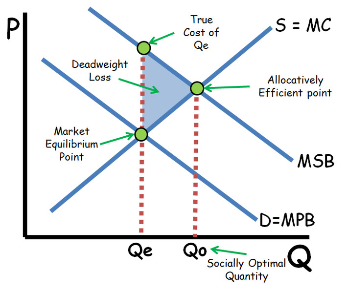
Positive externality and underproduction

On the graph:

• Demand = MPB
• MSB lies above MPB (vertical gap = marginal external benefit)
• Supply = MPC (in this case MPC = MSC because there is no production externality)

The market equilibrium occurs where MPB intersects supply, which is at a lower quantity than the socially optimal level.

Free market outcome:

• Where MPB = MPC
• Quantity is too low
• This is underproduction

Social optimum:

• Where MSB = MSC
• Higher quantity

The shaded triangle between the market quantity and the socially optimal quantity represents deadweight loss.

A per-unit subsidy equal to the marginal external benefit fixes this. It shifts supply down (or demand up) and increases output. Examples include public education funding and vaccine subsidies.

4. Other Policy Tools

Taxes and subsidies are common, but not the only tools.

• Environmental regulation (emissions limits, pollution caps)
• Public provision (government provides the good directly, like public schools)
• Property rights and the Coase Theorem
  If property rights are clearly assigned and transaction costs are low, private bargaining can solve the problem without government intervention.

Remember the 2017 AP FRQ with a monopoly and a negative externality. Same logic applies. You still find:

• Profit-maximizing output where MR = MPC
• Social optimum where MSC = MSB

Externalities can exist in monopoly, oligopoly, or perfect competition.

5. Free Riders and Non-Excludability

When a good is non-excludable, people cannot be prevented from using it.

That creates an incentive to free ride, meaning enjoy the benefit without paying.

Examples:

• Clean air
• National defense

This connects to positive externalities. If people can benefit without paying, private markets will underprovide the good.