Topic 5.4 Notes – Monopsonistic Markets
What a Monopsony Is in the Labor Market
A monopsony is a market with one buyer and many sellers. In labor markets, that means:
- One large firm hires most or all workers in a local area.
- The firm is a wage maker, not a wage taker.
- The market is imperfectly competitive.
- The firm faces the entire upward-sloping market supply curve of labor.
- Labor demand is still based on marginal revenue product (MRP), which comes from diminishing marginal returns.
Classic textbook example: a coal mining company in a company town. Historically, workers had few alternatives, so the mine had wage-setting power. Modern examples often include a large rural hospital system or a dominant employer like Amazon in a specific warehouse region.
Ground yourself in the competitive case:
- In perfect competition, firms are wage takers.
- There, MRC = wage = supply.
- In a monopsony, that equality breaks.
Labor Supply, MRC, and Why MRC Is Above Supply
Because the firm is the only buyer, it faces the market labor supply curve, which slopes upward.
Labor Supply
- Shows the wage workers are willing and able to accept.
- For the firm, this is also the average resource cost (ARC).
Marginal Resource Cost
MRC is the additional cost of hiring one more worker.
In a monopsony:
- To hire one more worker, the firm must offer a higher wage.
- It cannot wage discriminate. All workers must receive the same wage.
- So when the wage increases, the firm pays the higher wage to all existing workers.
That means:
This mirrors monopoly pricing:
- Monopoly → MR < Demand
- Monopsony → MRC > Supply
Here’s the standard graph you should picture. Notice the upward-sloping supply curve labeled S and the steeper MRC curve above it. That vertical gap between them is the extra cost created by having to raise wages for all workers when hiring one more.
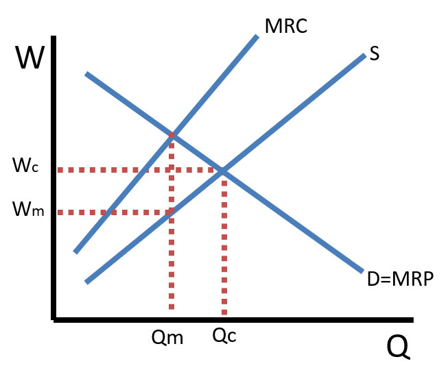
That vertical gap between MRC and Supply is one of the most tested ideas in this unit.
Profit-Maximizing Hiring and Wage
The hiring rule is the same structure as every factor market:
Step 1: Find Quantity of Labor
- Locate where MRP intersects MRC.
- That quantity is Qₘ, the monopsony level of employment.
Step 2: Find the Wage
- From Qₘ, move up to the Supply curve.
- That wage is Wₘ.
Workers are paid according to the supply curve, not MRC.
Key results:
- Wₘ < MRP at Qₘ
- Fewer workers are hired than in competition.
- Workers are paid less than their marginal revenue product.
If you get a table instead of a graph, calculate MRC carefully. Example:
If hiring the 4th worker raises wage from 15 dollars to 17 dollars and you already employ 3 workers, then:
You must include the wage increase paid to the first 3 workers. Students often forget that part.
Monopsony vs. Competitive Labor Market
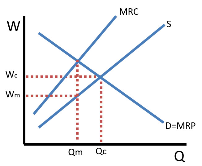
Use the graph below to see both outcomes on the same set of axes. The competitive equilibrium occurs where the labor supply curve intersects the labor demand curve (labeled D = MRP), giving wage Wc and quantity Qc. The monopsony outcome occurs where MRC intersects MRP, giving Qm, and the wage is then read off the supply curve at Wm.
| Feature | Perfect Competition | Monopsony |
|---|---|---|
| Buyers | Many firms | One firm |
| Wage | Wage taker | Wage maker |
| MRC | = Wage | Above Supply |
| Hiring rule | MRP = Wage | MRP = MRC |
| Wage level | Higher | Lower |
| Employment | Larger (Q꜀) | Smaller (Qₘ) |
Monopsony creates:
- Lower wages
- Underemployment
- Deadweight loss
This inefficiency is why labor economists study it so much.
Policy and Minimum Wage in a Monopsony
This is the twist that shows up on exams.
In a competitive market, a minimum wage above equilibrium reduces employment.
In a monopsony, a moderate minimum wage can:
- Increase wages
- Increase employment
If the minimum wage is set:
- Above Wₘ
- Below W꜀
Then the firm’s MRC becomes horizontal at the minimum wage (up to the supply quantity), and hiring increases.
This idea influenced debates about minimum wage policy, especially in research by David Card and Alan Krueger, who studied the effect of a minimum wage increase on fast-food employment in New Jersey and found that employment did not fall, contradicting the simple competitive model prediction. One interpretation is that monopsony power existed in those labor markets.
If the minimum wage is set too high, employment falls again.
Key Takeaways
Monopsony / Monopsonistic Labor Market
A labor market with one buyer of labor and many sellers of labor.
Characteristics of a Monopsony
Single large employer, imperfect competition, wage-making power, and upward-sloping labor supply to the firm.
Wage Maker
A firm with enough buying power to influence the wage it pays workers.
Labor Supply Curve to a Monopsonist
An upward-sloping curve showing higher wages are needed to attract more workers.
Marginal Revenue Product
The additional revenue generated by employing one more unit of labor.
Profit-Maximizing Hiring Rule in Monopsony
Hire labor until marginal revenue product equals marginal factor cost.
How to Find Wage and Quantity in a Monopsony Graph
Choose labor where MRP equals MFC, then read wage from the labor supply curve.
Monopsony Versus Competitive Labor Market
Monopsony hires where MRP = MFC and pays from supply; competition hires where MRP = supply.
Monopsony Outcome Relative to Competitive Labor Market
A monopsonist hires fewer workers and pays a lower wage than a competitive labor market.
Demand for Labor Equals MRP
The firm's labor demand curve is its marginal revenue product curve.
Minimum Wage in a Monopsony
A binding wage floor can raise wages and increase employment up to the relevant labor supply quantity.
Marginal Factor Cost in Monopsony
The cost of one more worker, including higher wages paid to all existing workers.
Notes
Monopsony / Monopsonistic Labor Market
A labor market with one buyer of labor and many sellers of labor.
Characteristics of a Monopsony
Single large employer, imperfect competition, wage-making power, and upward-sloping labor supply to the firm.
Wage Maker
A firm with enough buying power to influence the wage it pays workers.
Labor Supply Curve to a Monopsonist
An upward-sloping curve showing higher wages are needed to attract more workers.
Marginal Revenue Product
The additional revenue generated by employing one more unit of labor.
Profit-Maximizing Hiring Rule in Monopsony
Hire labor until marginal revenue product equals marginal factor cost.
How to Find Wage and Quantity in a Monopsony Graph
Choose labor where MRP equals MFC, then read wage from the labor supply curve.
Monopsony Versus Competitive Labor Market
Monopsony hires where MRP = MFC and pays from supply; competition hires where MRP = supply.
Monopsony Outcome Relative to Competitive Labor Market
A monopsonist hires fewer workers and pays a lower wage than a competitive labor market.
Demand for Labor Equals MRP
The firm's labor demand curve is its marginal revenue product curve.
Minimum Wage in a Monopsony
A binding wage floor can raise wages and increase employment up to the relevant labor supply quantity.
Marginal Factor Cost in Monopsony
The cost of one more worker, including higher wages paid to all existing workers.
