Topic 5.3 Notes – Profit-Maximizing Behavior in Perfectly Competitive Factor Markets
1. What a perfectly competitive labor market is
A factor market is where firms buy resources like labor, capital, and land. Here we focus on labor.
In a perfectly competitive labor market:
- Many firms are hiring workers (many buyers of labor).
- Many workers have identical skills (homogeneous labor).
- Firms are wage takers. No single firm can change the wage.
- Firms can hire as many workers as they want at the market wage.
Just like in perfect competition for goods, the market sets the price. Here, the “price” is the wage.
Market graph
The left panel shows the overall labor market, and the right panel shows a single firm that takes the market wage as given.
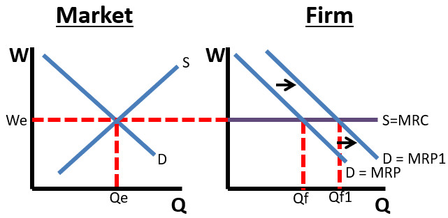
- DL slopes downward because of diminishing marginal returns. Each additional worker adds less to output, so each adds less revenue.
- SL slopes upward because higher wages encourage workers to give up leisure and work more.
- Equilibrium wage occurs where labor demand and labor supply intersect.
That equilibrium wage becomes the firm’s marginal resource cost (MRC), which is why the firm’s MRC curve in the right panel is horizontal at the market wage.
2. Marginal revenue product and the hiring rule
Marginal revenue product
The value of hiring one more worker is the marginal revenue product.
- MP = marginal physical product (extra output from one more worker)
- MR = marginal revenue from selling that output
If the firm is perfectly competitive in the product market, then . So:
This is also called the value of the marginal product of labor (VMPL).
Because MPL falls as more workers are hired, MRP is downward sloping. That curve is the firm’s demand for labor.
The firm’s hiring decision
In a perfectly competitive labor market:
- The firm faces a horizontal MRC curve at the market wage.
- So MRC = wage.
The graphs below show the market on the left setting the wage, and the individual firm on the right taking that wage as given and hiring where MRP equals MRC.
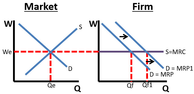
The firm hires workers where:
Or in plain language:
Hire workers as long as MRP ≥ wage, and stop when the next worker’s MRP would be less than the wage.
Quick calculation example
Suppose:
- Wage = 20 dollars
- Output price = 5 dollars
| Workers | MPL | MRP (= MPL × 5) |
|---|---|---|
| 1 | 8 | 40 |
| 2 | 6 | 30 |
| 3 | 4 | 20 |
| 4 | 3 | 15 |
The firm hires 3 workers.
The 4th worker’s MRP (15) is less than the wage (20), so that worker is not hired.
This exact type of table shows up on AP questions. Multiply carefully and compare to the wage. Don’t overthink it.
3. Connecting the market and firm graphs
On the AP exam, these are often drawn side by side. You are expected to move from the market to the firm without hesitation.

Competitive labor market and individual firm hiring decision
On the left is the labor market. Supply and demand intersect to determine the equilibrium wage.
The dashed horizontal line carries that wage over to the individual firm on the right.
- The firm takes the wage as given.
- That wage becomes the horizontal MRC line.
- The firm hires where MRP = MRC.
Example change
If labor supply increases (immigration, more college grads, etc.):
- Market wage falls.
- On the firm graph, the horizontal MRC line shifts downward.
- Each firm hires more workers.
If labor demand increases (higher product demand increases MRP):
- Market wage rises.
- The horizontal MRC line shifts upward on the firm graph.
- Each firm’s MRP curve also shifts right (since MRP rose), so firms hire more workers at the new equilibrium despite the higher wage.
A common mistake is shifting the MRP curve when the wage changes. Wage changes shift MRC, not MRP.
4. Cost minimization and the least-cost rule
When firms use multiple inputs, like labor and capital, they want the cheapest combination that produces a given output.
The least-cost rule:
- = marginal product of each input
- = price of each input
The last dollar spent on each input must produce the same marginal product.
If:
- → hire more labor.
- → hire more capital.
This is the producer version of utility maximization from Unit 1.
Isoquants and isocost lines explain this graphically, but those graphs are beyond AP scope.
5. Profit maximization with multiple inputs
To maximize profit, the firm applies the same idea to each resource:
For labor:
- Hire where
For capital:
- Hire where
When this holds for every input:
- The last worker and the last machine both add exactly as much revenue as they cost.
This connects to the bigger idea in PRD-4: factor prices send signals. High wages signal scarce labor. Firms respond by hiring less or substituting capital. That’s how competitive markets allocate resources efficiently.
Key Takeaways
Perfectly Competitive Labor Market Characteristics
Many firms hire identical workers, each firm is a wage taker, and labor is hired at the market wage.
Market Labor Demand and Supply
Labor demand slopes downward from diminishing marginal returns, while labor supply slopes upward as higher wages attract more work.
Wage Taker
A firm that must accept the market wage because its hiring is too small to affect it.
Marginal Resource Cost
The additional cost of hiring one more unit of a resource; in a competitive labor market, it equals the wage.
Individual Firm Labor Market Graph
A downward-sloping marginal revenue product curve intersects a horizontal marginal resource cost curve at the profit-maximizing quantity of labor.
Side-by-Side Labor Market and Firm Graphs
Changes in market labor supply or demand change the equilibrium wage, which shifts each firm's horizontal marginal resource cost curve.
Least-Cost Rule
Use inputs so the marginal product per dollar spent is equal across all resources.
Profit-Maximizing Combination of Resources
Choose each input so its marginal revenue product equals its marginal resource cost.
Marginal Revenue Product and Value of Marginal Product
The extra revenue from one more worker; in competitive output markets, it equals MPL times price.
Profit-Maximizing Hiring Rule
Hire workers until marginal revenue product equals wage, using MPL times MR or price.
Perfectly Elastic Labor Supply to the Firm
An individual firm can hire any number of workers at the market wage.
Notes
Perfectly Competitive Labor Market Characteristics
Many firms hire identical workers, each firm is a wage taker, and labor is hired at the market wage.
Market Labor Demand and Supply
Labor demand slopes downward from diminishing marginal returns, while labor supply slopes upward as higher wages attract more work.
Wage Taker
A firm that must accept the market wage because its hiring is too small to affect it.
Marginal Resource Cost
The additional cost of hiring one more unit of a resource; in a competitive labor market, it equals the wage.
Individual Firm Labor Market Graph
A downward-sloping marginal revenue product curve intersects a horizontal marginal resource cost curve at the profit-maximizing quantity of labor.
Side-by-Side Labor Market and Firm Graphs
Changes in market labor supply or demand change the equilibrium wage, which shifts each firm's horizontal marginal resource cost curve.
Least-Cost Rule
Use inputs so the marginal product per dollar spent is equal across all resources.
Profit-Maximizing Combination of Resources
Choose each input so its marginal revenue product equals its marginal resource cost.
Marginal Revenue Product and Value of Marginal Product
The extra revenue from one more worker; in competitive output markets, it equals MPL times price.
Profit-Maximizing Hiring Rule
Hire workers until marginal revenue product equals wage, using MPL times MR or price.
Perfectly Elastic Labor Supply to the Firm
An individual firm can hire any number of workers at the market wage.
