Topic 2.6 Notes – Market Equilibrium and Consumer and Producer Surplus

1. Market Equilibrium

A market equilibrium happens where quantity demanded equals quantity supplied. In symbols, $Q_{d} = Q_{s}$. This point gives you the equilibrium price (P_{e}) and equilibrium quantity (Q_{e}).

Here’s what that looks like on a standard supply and demand graph:

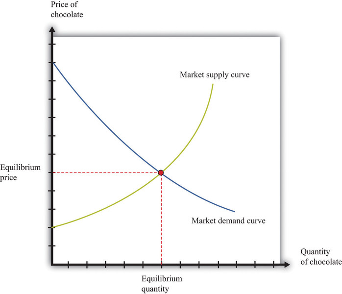
Supply and demand at equilibrium

The downward-sloping demand curve and upward-sloping supply curve intersect at the red point. The dashed lines show the equilibrium price on the vertical axis and the equilibrium quantity on the horizontal axis.

At $P_{e}$ and $Q_{e}$:

• Buyers purchase exactly what sellers produce.
• There is no shortage ($Q_{d} > Q_{s}$).
• There is no surplus ($Q_{s} > Q_{d}$).

Why equilibrium is stable

The market has a built-in correction process:

• Price above equilibrium → surplus
  • Unsold goods pile up.
  • Firms lower price.
  • Quantity demanded rises, quantity supplied falls.
  • Market moves back to $P_{e}$.
• Price below equilibrium → shortage
  • Buyers compete for limited goods.
  • Price gets bid up.
  • Quantity demanded falls, quantity supplied rises.
  • Market returns to $P_{e}$.

This self-correcting mechanism is why economists say competitive markets “clear.”

Why equilibrium matters

The equilibrium price sends a signal.

• To producers: how much to produce.
• To consumers: how scarce the good is.

When housing prices surge in a city, that price signal tells builders demand is strong and supply is limited. In a perfectly competitive market, this equilibrium also creates allocative efficiency, meaning resources go to their highest-valued use.

2. Consumer Surplus and Producer Surplus

Economists measure market benefits using economic surplus.

Consumer Surplus (CS)

Consumer surplus is the difference between what buyers are willing to pay and what they actually pay.

For one person:

$$\text{Individual CS} = \text{maximum willingness to pay} - \text{market price}$$

If you would pay 500 dollars for concert tickets but buy them for 350 dollars, your CS is 150 dollars.

On a standard supply and demand graph, CS is the triangle above the equilibrium price and below the demand curve:

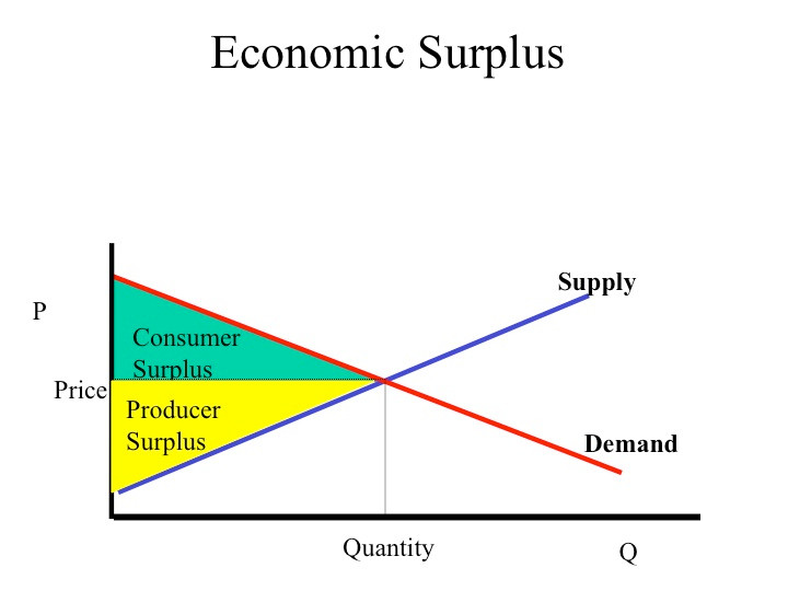
The demand curve represents marginal benefit or willingness to pay. Anyone whose willingness to pay is above the market price gains surplus.

Producer Surplus (PS)

Producer surplus is the difference between what sellers are willing to accept and what they actually receive.

For one firm:

$$\text{Individual PS} = \text{market price} - \text{minimum acceptable price}$$

If a firm would sell a product for 20 dollars but receives 35 dollars, its PS is 15 dollars per unit.

On the same type of graph, PS is the triangle below the equilibrium price and above the supply curve:

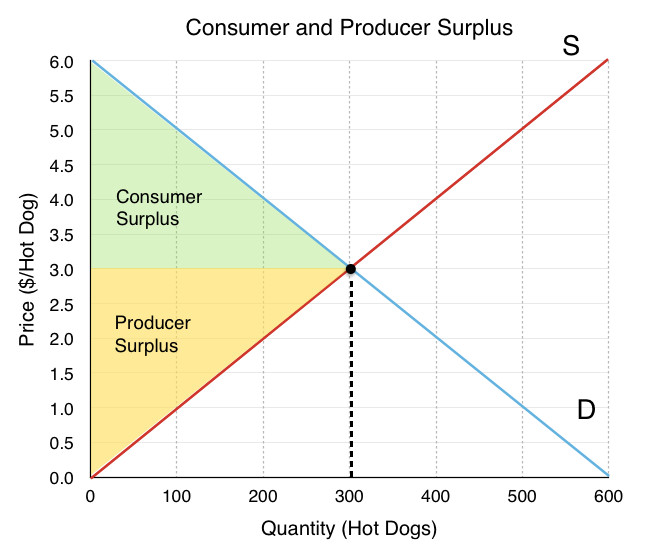
The supply curve reflects marginal cost. When price is above marginal cost, firms gain surplus.

Total Economic Surplus

$$\text{Total Surplus} = \text{Consumer Surplus} + \text{Producer Surplus}$$

Graphically, it’s the entire area between demand and supply up to $Q_{e}$. This measures the total gains from voluntary exchange.

3. Calculating Consumer and Producer Surplus

On tests, you’ll calculate triangle areas from graphs or tables.

Most of the time, CS and PS are triangles.

$$\text{Area} = \tfrac{1}{2} \times \text{base} \times \text{height}$$

For consumer surplus:

• Base = $Q_{e}$
• Height = demand intercept − $P_{e}$

For producer surplus:

• Base = $Q_{e}$
• Height = $P_{e}$ − supply intercept

Example

Suppose:

• Demand intercept = 30 dollars
• Supply intercept = 10 dollars
• $P_{e} = 18$ dollars
• $Q_{e} = 40$

Consumer surplus:

$$\tfrac{1}{2} \times 40 \times (30 - 18) = 240$$

Producer surplus:

$$\tfrac{1}{2} \times 40 \times (18 - 10) = 160$$

Watch this common mistake: students sometimes use the wrong price for height. Always use the vertical distance to the intercept, not just any point on the curve.

If given a table, find where $Q_{d} = Q_{s}$, then compute surplus per unit and add them up.

4. Why Market Equilibrium Is Efficient

At equilibrium:

• Marginal benefit = marginal cost
• Every mutually beneficial trade occurs.
• Total economic surplus is maximized.

If output is above $Q_{e}$, then $MC > MB$. That’s overproduction.
If output is below $Q_{e}$, then $MB > MC$. That’s underproduction.

This condition is called allocative efficiency.

Price controls show what happens when we move away from equilibrium. A binding rent ceiling creates a shortage and reduces total surplus. The competitive equilibrium, assuming no externalities or other market failures, is the socially optimal quantity.