Topic 1.5 Notes – Cost-Benefit Analysis
1. Opportunity cost and total economic cost
Opportunity cost is the value of the next best alternative given up when you make a choice. Because you can’t do everything, choosing one option means giving up something else.
If you go to college instead of working a 25,000-dollar job, that lost salary is part of the opportunity cost. If a government spends money on highways instead of schools, the foregone school funding is the opportunity cost. Same logic everywhere.
Explicit vs. implicit costs
Opportunity cost includes both explicit and implicit costs.
| Explicit Costs | Implicit Costs | |
|---|---|---|
| What they are | Out-of-pocket monetary payments | Value of forgone alternatives (no money paid) |
| Examples | Tuition, rent, wages paid to workers, materials | Wages you could have earned, interest you could have earned on savings, using your own building instead of renting it out |
| Recorded in accounting? | Yes | No |
Total economic cost = explicit costs + implicit costs
Two common mistakes on quizzes:
- Only include costs that change because of the decision. If you’ll pay for food either way, that’s not part of the opportunity cost.
- The opportunity cost is the highest-valued alternative, not every alternative combined.
When asked to calculate opportunity cost, literally add up the relevant explicit and implicit costs. That’s it.
2. Total benefits, total costs, and net benefits
Now zoom out to the full decision.
- Total benefit (TB)
- For consumers → measured in utility (satisfaction)
- For firms → measured as total revenue
- Total cost (TC) = total economic cost of producing or consuming that quantity.
The key equation:
The rational choice is the one that maximizes total net benefits.
What this looks like on a graph
Look at the graph and focus on the vertical distance between the total benefit and total cost curves.
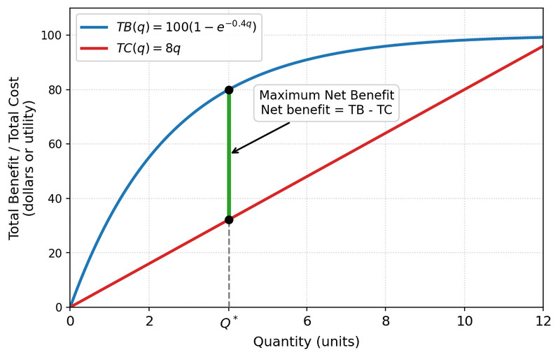
Total benefit and total cost with maximum net benefit at Q*
At low quantities, TB rises faster than TC. Net benefit increases.
At some point, the vertical gap between TB and TC is largest. That’s the optimal quantity .
After that, TC catches up and net benefit shrinks.
On a table question, you:
- List quantities.
- Calculate TB and TC at each level.
- Subtract to find net benefit.
- Choose the quantity with the highest net benefit.
If net benefit turns negative, you’ve gone too far.
This “compare totals” method is often used for all-or-nothing decisions, like building a bridge or not.
3. Marginal analysis and the MB = MC rule
Most decisions can be broken into smaller steps. That’s where marginal thinking comes in.
- Marginal benefit (MB) = extra benefit from one more unit.
- Marginal cost (MC) = extra cost of one more unit.
- Per-unit surplus =
The cost-benefit maximizing principle
The rule:
Think through the three cases:
- MB > MC → you’re gaining more than you’re giving up. Keep going.
- MB < MC → the extra unit reduces net benefit. Stop.
- MB = MC → you’re at the optimal quantity.
If there’s no exact equality, choose the last unit where .
Law of diminishing marginal utility
As you consume more of a good, marginal benefit eventually falls.
First slice of pizza has high utility. Third slice gives less. Eventually MB can hit zero or even become negative. That’s the law of diminishing marginal utility, and it explains why the MB curve slopes downward.
Here’s what that looks like on the standard MB-MC graph.
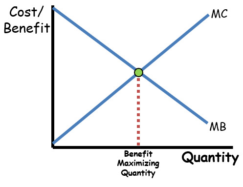
Marginal benefit and marginal cost at the optimal quantity
At the green dot, MB and MC intersect. The dashed line shows the benefit-maximizing quantity.
To the left of the intersection, MB > MC.
To the right, MB < MC.
On multiple-choice questions, the College Board loves giving you a table of MB values and a constant price (which equals MC for a price-taking consumer). You pick the last unit where MB is at least as large as price.
4. When to use total vs. marginal analysis
Use marginal analysis when:
The decision can be adjusted unit by unit.
Examples:
- How many hours to work?
- How many units to produce?
- How many cups of coffee to buy?
You only need to compare MB and MC.
Use total analysis when:
The decision is all-or-nothing.
Examples:
- Attend college or not.
- Build a factory or not.
- Fund a public project or not.
In those cases, compare total benefits to total costs and choose the higher net benefit.
Key Takeaways
Cost-Benefit Analysis
A decision method that compares expected total benefits with total costs.
Opportunity Cost
The value of the next best alternative given up when a choice is made.
Explicit and Implicit Costs
Direct out-of-pocket payments versus forgone income or benefits from using resources differently.
Total Benefit and Total Cost
The full satisfaction or revenue gained and the full economic cost incurred at a given choice.
Utility
The satisfaction or benefit a consumer receives from consuming goods or services.
Marginal Benefit and Marginal Cost
The additional benefit and additional cost from one more unit of a good or activity.
Law of Diminishing Marginal Utility
As consumption rises, each additional unit eventually provides less extra satisfaction than the previous one.
Net Benefits
The difference between total benefits and total costs.
Optimal Choice
The decision or quantity that produces the greatest net benefit.
Cost-Benefit Maximizing Principle
Choose the quantity where marginal benefit equals marginal cost, or the last unit before marginal benefit falls below marginal cost.
Total Revenue
The total money a firm receives from selling its output.
Notes
Cost-Benefit Analysis
A decision method that compares expected total benefits with total costs.
Opportunity Cost
The value of the next best alternative given up when a choice is made.
Explicit and Implicit Costs
Direct out-of-pocket payments versus forgone income or benefits from using resources differently.
Total Benefit and Total Cost
The full satisfaction or revenue gained and the full economic cost incurred at a given choice.
Utility
The satisfaction or benefit a consumer receives from consuming goods or services.
Marginal Benefit and Marginal Cost
The additional benefit and additional cost from one more unit of a good or activity.
Law of Diminishing Marginal Utility
As consumption rises, each additional unit eventually provides less extra satisfaction than the previous one.
Net Benefits
The difference between total benefits and total costs.
Optimal Choice
The decision or quantity that produces the greatest net benefit.
Cost-Benefit Maximizing Principle
Choose the quantity where marginal benefit equals marginal cost, or the last unit before marginal benefit falls below marginal cost.
Total Revenue
The total money a firm receives from selling its output.
