Topic 3.2 Notes – Short-Run Production Costs

1. Short Run Production and the Structure of Costs

In the short run, at least one input is fixed. Usually that’s capital like buildings or machines. Labor is typically variable. In the long run, all inputs are variable.

Because something is fixed in the short run, firms face two types of costs.

Types of Costs

• Fixed Cost (FC)
  • Does not change with output.
  • Exists even at $Q = 0$.
  • Examples: rent, insurance, salaried managers.
  • Graphically: a horizontal line.
• Variable Cost (VC)
  • Changes as output changes.
  • Examples: hourly labor, raw materials.
  • Rises as output rises.
• Total Cost (TC)

  $$TC = FC + VC$$

  • Increases as output increases.
  • The vertical distance between TC and VC equals FC.

Here’s what that looks like on a graph of output (jackets per day) and cost per day:

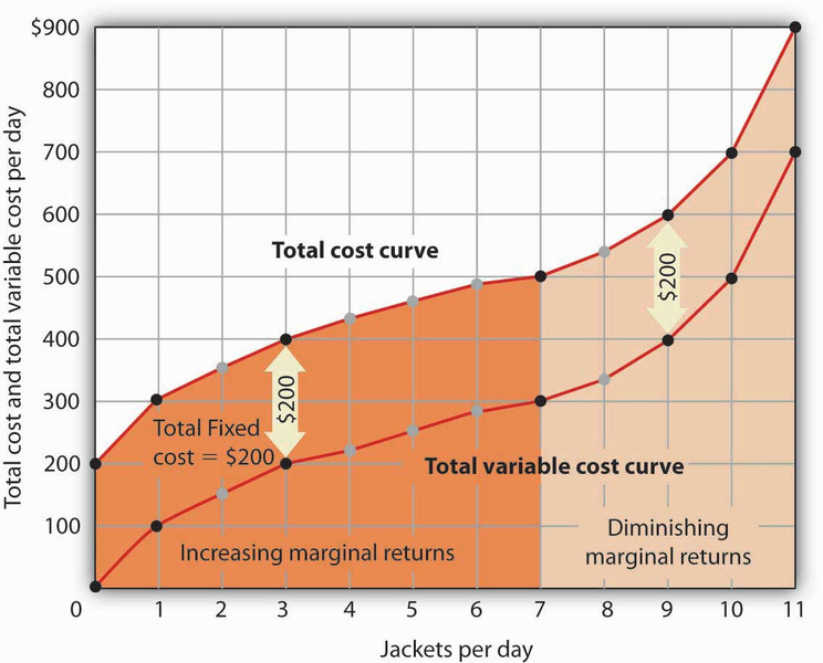
Total cost and total variable cost in the short run

Notice that the total cost curve always lies above the total variable cost curve. The vertical gap between them is constant at 200 dollars, which represents total fixed cost. Even at zero output, total cost is 200 dollars because fixed cost must be paid.

Important rule: FC is constant at all output levels. VC and TC rise as output rises.

Economic vs Accounting Cost

• Accounting cost = explicit payments.
• Economic cost = explicit + implicit (opportunity cost).

On the AP exam, when they say “cost,” they mean economic cost unless stated otherwise.

2. Per-Unit and Marginal Costs

Once we know total costs, we convert them into per-unit and marginal measures.

Average Costs

• AFC $= \frac{FC}{Q}$
• AVC $= \frac{VC}{Q}$
• ATC $= \frac{TC}{Q}$

Because $TC = FC + VC$,
$$ATC = AVC + AFC$$

Shapes

• AFC
  • Always downward sloping.
  • As Q increases, fixed cost is spread over more units.
  • Approaches zero but never touches it.
• AVC and ATC
  • U-shaped.
  • Fall at first, then rise.

Marginal Cost

$$MC = \frac{\Delta TC}{\Delta Q}$$

MC is the cost of producing one more unit. Since fixed cost doesn’t change, MC is driven by changes in variable cost.

The Key Relationship

• If MC < ATC, ATC falls.
• If MC > ATC, ATC rises.
• MC intersects ATC and AVC at their minimum points.

Think GPA. A grade below your average pulls it down. Above pulls it up.

This is the standard short-run cost graph you should be able to sketch from memory:

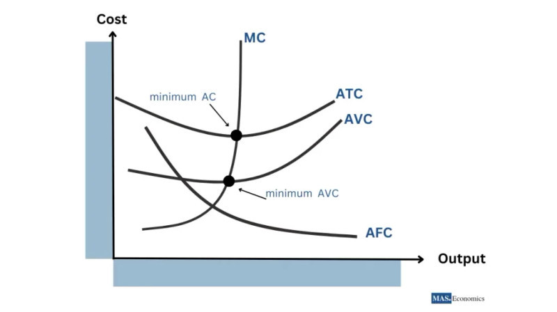
Short-run cost curves: MC, ATC, AVC, and AFC

3. Why Cost Curves Are Shaped This Way

Everything comes from the law of diminishing marginal returns.

As you add more variable labor to fixed capital:

1. Specialization and division of labor
   • Workers become more efficient.
   • Marginal product rises.
   • MC falls.
2. Diminishing marginal returns
   • Crowding and inefficiency set in.
   • Marginal product falls.
   • MC rises.

Critical Link

• When marginal product rises → MC falls.
• When marginal product falls → MC rises.

Because diminishing marginal returns eventually happen in the short run, the MC curve slopes upward.

That upward-sloping MC later becomes the firm’s supply curve in perfect competition. This connection shows up all over Unit 3.

4. Shifts in Cost Curves

Cost curves shift when input prices or productivity change.

Change in Fixed Costs

If rent increases:

• AFC shifts up.
• ATC shifts up.
• AVC and MC do not shift.

Why? Fixed cost does not affect the cost of the next unit.

Change in Variable Costs (like wages)

If wages rise:

• MC shifts up.
• AVC shifts up.
• ATC shifts up.
• AFC does not shift.

Real-world anchor:

• During COVID-19 supply chain disruptions, higher shipping and materials costs raised firms’ variable costs. That shifted MC, AVC, and ATC upward.

Productivity Improvements

If workers become more productive:

• Marginal product rises.
• MC shifts down.
• AVC and ATC shift down.

Automation in manufacturing is a classic example.

5. Calculations You Must Be Able to Do

From a table:

• Compute $TC = FC + VC$.
• Compute AFC, AVC, ATC.
• Compute $MC = \frac{\Delta TC}{\Delta Q}$.

Example:

If TC at 4 units is 120 dollars and TC at 5 units is 140 dollars:

$$MC = \frac{140 - 120}{1} = 20$$

You should be able to:

• Identify minimum ATC and AVC.
• Spot where MC intersects them.
• Determine which curves shift when costs change.

Tables, graphs, and formulas are the same story told three ways.