Topic 3.3 Notes – Long-Run Production Costs

1. The Long Run in Production and Cost

In the long run, all inputs are variable. Labor, capital, land, entrepreneurship. Nothing is fixed.

In the short run, at least one input is fixed, which gives us fixed costs and those familiar SRATC curves. In the long run:

• There are no fixed costs
• Firms can change plant size
• Firms can enter or exit industries
• Firms can fully adjust production methods

That flexibility is the whole point. A firm is no longer stuck on one short-run average total cost curve.

Long-Run Average Total Cost (LRATC)

The LRATC shows the lowest possible average total cost for each output level when all inputs are variable.

Think of it as the “best choice” curve. At every quantity, the firm picks the plant size that minimizes cost.

Here’s what that looks like:

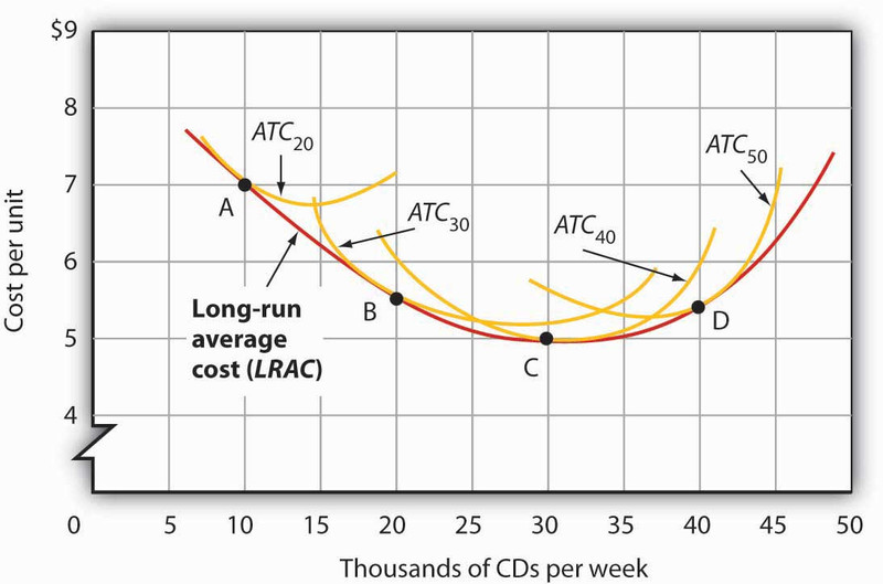
Short-run ATC curves and the long-run average cost (LRAC) envelope

Key details to understand:

• Each SRATC represents a different plant size.
• The LRATC is the lower envelope of those SRATC curves.
• The LRATC is tangent to each SRATC curve (not necessarily at its minimum point, except at minimum efficient scale).
• The LRATC is flatter than any one SRATC because firms can adjust scale.

On a quiz, if they ask why a firm isn’t stuck at high cost in the long run, the answer is simple: it can change plant size.

2. Returns to Scale

Returns to scale describe what happens when all inputs change proportionally.

If a firm doubles all inputs:

Increasing Returns to Scale

• Output more than doubles
• Example: Inputs ×2 → Output ×2.6
• Per-unit cost falls
• Corresponds to downward-sloping LRATC

Constant Returns to Scale

• Output exactly doubles
• Inputs ×2 → Output ×2
• Per-unit cost stays constant
• Corresponds to flat LRATC

Decreasing Returns to Scale

• Output less than doubles
• Inputs ×2 → Output ×1.5
• Per-unit cost rises
• Corresponds to upward-sloping LRATC

AP questions love giving a table like:

• Labor: 10 → 20
• Capital: 5 → 10
• Output: 100 → 240

Since output more than doubles, that’s increasing returns to scale.

Be careful not to confuse this with diminishing marginal returns, which is a short-run concept with one fixed input.

3. Economies and Diseconomies of Scale

Returns to scale explain the shape of the LRATC.

Economies of Scale

When output increases and average cost falls, the firm is experiencing economies of scale.

Common causes:

• Specialization of labor and management
• Bulk purchasing discounts
• Spreading startup costs over more units
• Access to better technology

This is why companies like Amazon or large automobile manufacturers can produce at lower per-unit cost than small firms.

Constant Returns to Scale

At some output, the firm reaches its efficient scale. Increasing output no longer lowers cost. LRATC is flat here.

Diseconomies of Scale

When output increases and average cost rises, the firm faces diseconomies of scale.

Causes:

• Coordination problems
• Communication breakdown
• Bureaucratic inefficiency

Large corporations sometimes struggle with this as they grow too complex.

Put it all together and you get the typical U-shaped long-run average total cost curve:

Long-run average total cost curve with economies, constant returns, and diseconomies of scale

4. Minimum Efficient Scale and Market Structure

The Minimum Efficient Scale (MES) is the lowest level of output at which the LRATC reaches its minimum.

It’s the smallest quantity where a firm fully exploits economies of scale.

Why this matters:

• Small MES relative to market demand
  Many firms can operate efficiently → competitive markets (restaurants, clothing stores).
• Large MES relative to demand
  Only a few firms can reach low cost → oligopoly (airlines, car manufacturers).
• MES nearly equals total market demand
  One firm can supply the market at lowest cost → natural monopoly (utilities like water or electricity distribution).

Cost structure helps determine market structure. That connection shows up later in perfect competition, monopoly, and oligopoly.

5. Calculations and Graph Skills

You should be comfortable calculating:

$$\text{ATC} = \frac{\text{Total Cost}}{\text{Quantity}}$$

If total cost is 900 and output is 300 units, ATC = 3 dollars per unit.

From a data table, compare how output changes when inputs change proportionally to determine returns to scale.

From a graph, be able to:

• Identify LRATC vs SRATC
• Locate MES
• Classify regions as economies or diseconomies
• Explain why LRATC is flatter than SRATC

On FRQs, they often want a clear sentence like: “Because output increased more than inputs, the firm experiences increasing returns to scale.”