Topic 6.4 Notes – The Effects of Government Intervention in Different Market Structures

1. Per-Unit Taxes and Subsidies in Competitive and Imperfect Markets

A per-unit tax is a tax on every unit produced or sold. A per-unit subsidy is a payment for every unit produced.

Because it applies to each unit, it changes marginal cost (MC).

How They Shift Curves

• Per-unit tax
  • MC shifts up by the amount of the tax.
  • In perfect competition → supply shifts left.
  • In monopoly or monopolistic competition → the firm’s MC curve shifts up.
  • ATC also shifts up (variable cost increased).
• Per-unit subsidy
  • MC shifts down.
  • Supply shifts right in perfect competition.
  • ATC shifts down.

If MC changes, the firm’s profit-maximizing output changes. That’s the core idea.

What Changes in the Market

Here’s the standard competitive market tax diagram you should picture. Focus on the shift from the original supply curve to the upward-shifted curve labeled S + Tax:

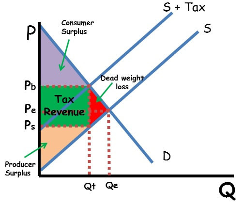
Per-unit tax in a competitive market

With a per-unit tax:

• Price consumers pay (Pb) rises
• Price producers receive (Ps) falls
• Quantity decreases from Qe to Qt
• Consumer surplus decreases
• Producer surplus decreases
• Government revenue = tax × quantity sold (the rectangle labeled Tax Revenue)
• Deadweight loss from underproduction (the red triangle)

With a subsidy:

• Consumers pay less.
• Producers receive more.
• Quantity increases.
• Government spending = subsidy × quantity.
• DWL from overproduction.

You might get a graph or table and be asked to calculate tax revenue. For example, if the tax is 3 dollars per unit and 80 units are sold after the tax, revenue is $3 \times 80 = 240$ dollars. Straight rectangle.

Tax Incidence and Elasticity

Who “pays” more depends on elasticity.

• More inelastic demand → consumers bear more of the burden.
• More inelastic supply → producers bear more.

Gasoline taxes are a classic example. Demand for gas is relatively inelastic in the short run, so consumers absorb most of the tax. Cigarette taxes work similarly and are often used both to raise revenue and reduce consumption.

On a graph, the steeper curve bears more of the tax. That’s an easy MCQ favorite.

2. Lump-Sum Taxes and Subsidies

A lump-sum tax is a fixed amount regardless of output. Think of a flat 500-dollar tax on a firm.

This changes fixed costs only.

• MC does not change
• MB does not change
• Only ATC shifts up (or down for subsidy)

That means output stays the same in the short run.

• Perfect competition → same quantity, lower profit. In the long run, firms may exit.
• Monopoly → same $MR = MC$ output and same price, just lower profit.

If MC doesn’t move, output doesn’t move. That line alone answers a lot of FRQs.

3. Price Controls in Different Market Structures

A binding price ceiling is below equilibrium.
A binding price floor is above equilibrium.

Perfect Competition

In a competitive market, a binding ceiling creates a shortage and a binding floor creates a surplus.

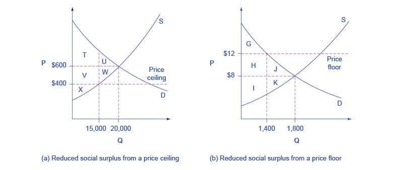
Binding price ceiling and price floor in perfect competition

• Ceiling → shortage (Qd > Qs)
• Floor → surplus (Qs > Qd)
• Creates deadweight loss
• Quantity exchanged equals the smaller of Qd or Qs

Monopoly Regulation

Unregulated monopoly produces where MR = MC and charges price from the demand curve. This creates DWL because $P > MC$.

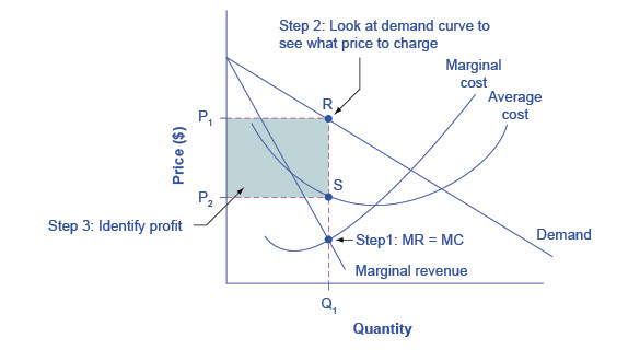
Monopoly profit maximization and regulation points

Governments regulate monopolies two main ways:

Socially Optimal Price $P = MC$

• Eliminates DWL (allocative efficiency).
• Often $P < ATC$ → firm incurs losses.
• Requires a lump-sum subsidy to keep firm operating.
• Common in natural monopolies like electricity and water utilities.

Fair-Return Price $P = ATC$

• Firm earns zero economic profit.
• Less DWL than unregulated monopoly.
• No subsidy needed.
• Output higher than monopoly level, but less than socially optimal.

You should be able to identify both on a graph quickly.

Monopsony and Minimum Wage

A monopsony hires where MRP = MRC, paying a wage below competitive equilibrium.

A binding price floor (minimum wage) set between the monopsony wage and the competitive wage can:

• Increase wages
• Increase employment

This is different from perfect competition, where a price floor creates unemployment.

4. Regulating Monopoly and Natural Monopoly

A natural monopoly has downward-sloping ATC due to economies of scale. One firm can produce at lower cost than multiple firms.

On the graph below, notice that the ATC curve falls over a large range of output. That cost structure is what makes regulation necessary.

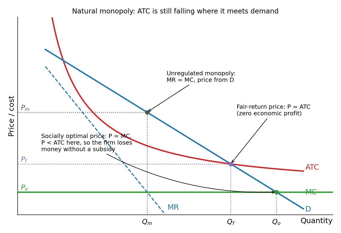
Natural monopoly: unregulated (MR = MC), fair-return (P = ATC), and socially optimal (P = MC) outcomes

To force $P = MC$:

• Firm produces efficiently.
• But $ATC > MC$ at that quantity.
• Firm loses money.
• Government must provide a lump-sum subsidy.

At the quantity where demand intersects MC, price is below ATC, which means losses without government support.

Many utilities operate this way.

5. Antitrust Policy and Increasing Competition

Governments also use antitrust policy to promote competition:

• Break up firms (AT&T in the 1980s).
• Block mergers.
• Ban anti-competitive practices.

Goal:

• Increase output.
• Lower price.
• Reduce DWL.
• Move market closer to competitive outcome.

Collusion graphs are outside AP scope, but you should know the idea that more competition usually reduces inefficiency.