Topic 5.2 Notes – Changes in Factor Demand and Factor Supply

1. How Factor Markets Work

A factor market is where firms demand resources and households supply them. In Unit 5, that resource is mostly labor.

• Labor demand (LD) → downward sloping
  Higher wage → firms hire fewer workers.
• Labor supply (LS) → upward sloping
  Higher wage → more people are willing to work.

Economists often label labor as N (for “number of workers”), but L is fine on the AP exam.

Here’s the standard picture:

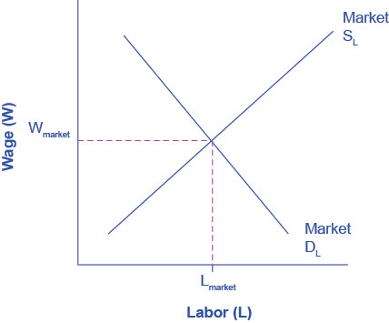
Market for labor at equilibrium

At equilibrium:

• Quantity of labor demanded = quantity supplied
• No labor shortage
• No labor surplus (unemployment caused by wage being too high)

If the wage is:

• Above equilibrium → surplus of labor (unemployment), like with a binding minimum wage.
• Below equilibrium → shortage of labor (rare, but would happen with a binding maximum wage).

This topic is about shifts of LD and LS, not movements along them.

2. What Shifts Labor Demand

Labor demand is derived demand. Firms hire workers because workers help produce goods and services that consumers want.

The key idea underneath all of this is:

$$\text{MRP} = \text{MP} \times \text{Price of Output}$$

If a worker generates more revenue, firms want more of that worker.

1. Changes in Product Demand

If demand for the final good increases:

• Output price rises
• Workers generate more revenue
• Labor demand shifts right

Example:

• During World War II, demand for military equipment soared → huge increase in demand for factory workers.

If demand for the product falls:

• Labor demand shifts left
• Example: decline in print newspapers → fewer print journalists hired.

Be careful: this is a shift because the product demand changed, not the wage.

2. Changes in Productivity

If workers become more productive:

• Each worker produces more output
• Marginal revenue product rises
• LD shifts right

Causes:

• New technology
• Better training or education
• More or better capital (tools, machines)

Example:

• Assembly line innovation in the early 20th century increased factory productivity → firms demanded more labor.

If productivity falls, LD shifts left.

3. Prices of Related Inputs

Think in terms of substitutes and complements.

Substitute Inputs

If the price of a substitute rises:

• Firms switch toward labor
• LD shifts right

Example:

• If industrial robots become more expensive, firms hire more workers.

If substitute price falls:

• Firms replace workers with machines
• LD shifts left

Complementary Inputs

If the price of a complement rises:

• Production becomes more expensive
• Firms reduce both inputs
• LD shifts left

Example:

• If aluminum prices rise sharply, soda production may fall → fewer bottling plant workers needed.

3. What Shifts Labor Supply

Labor supply reflects workers’ willingness and ability to work at different wages.

1. Number of Qualified Workers

More qualified workers → LS shifts right
Fewer qualified workers → LS shifts left

Examples:

• Increase in engineering graduates → LS right for engineers
• Stricter immigration laws → LS left in affected industries

Immigration is a classic AP example. An increase in immigration typically increases labor supply.

2. Education and Licensing

If government makes it harder to enter a profession:

• Fewer workers qualify
• LS shifts left

Example:

• Stricter licensing requirements for electricians reduce supply.

If barriers are lowered:

• LS shifts right.

3. Preferences, Culture, and Wealth

Labor supply depends on social norms and incentives.

Examples:

• During World War II, many women entered the workforce → LS shifted right.
• Greater preference for leisure → LS shifts left.
• Wealth effect: if long-term wealth increases, people work less at every wage → LS shifts left.

Also:

• Better working conditions → LS right.
• More attractive alternative jobs → can shift LS out of a specific industry.

4. How Shifts Change Wage and Employment

When curves shift, both wage and employment change.

In the graph below, labor demand stays fixed and labor supply shifts to the right. Notice what happens to equilibrium: wage falls from the higher dashed level to the lower one, and employment rises from the left quantity to the right quantity.

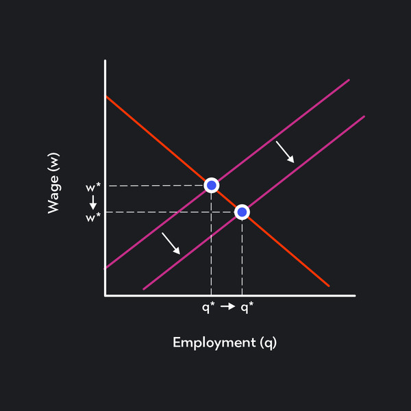
Increase in labor supply

Memorize these patterns:

• Increase in LD → wage ↑, employment ↑
• Decrease in LD → wage ↓, employment ↓
• Increase in LS → wage ↓, employment ↑
• Decrease in LS → wage ↑, employment ↓

On FRQs, don’t stop at “curve shifts right.” Explain the incentive story. Higher output price raises MRP, which increases demand for workers. Higher wages attract more workers because labor supply slopes upward. Wages send signals and create incentives. That’s the core logic of this whole unit.