Topic 1.2 Notes – Opportunity Cost and the Production Possibilities Curve (PPC)
1. What the Production Possibilities Curve Is
The Production Possibilities Curve (PPC) shows all the possible combinations of two goods an economy can produce when it uses its resources fully and efficiently.
We assume:
- Only two goods
- Fixed resources (land, labor, capital, entrepreneurship)
- Fixed technology
- The economy is at full employment unless shown otherwise
Here’s what a standard PPC looks like:
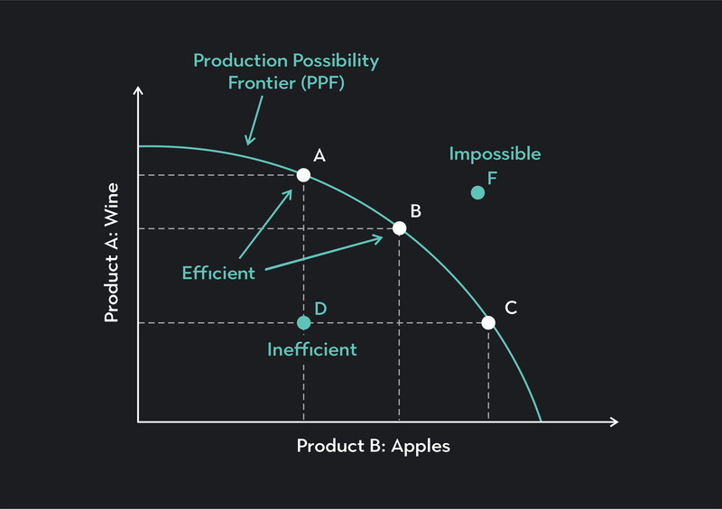
Production Possibilities Curve (PPC)
What the Points Mean
- On the curve → Productive efficiency (all resources fully used)
- Inside the curve → Inefficiency (unemployment, recession, underused resources)
- Outside the curve → Unattainable with current resources/technology
The PPC exists because of scarcity. Resources are limited, so producing more of one good means giving up some of another.
2. Opportunity Cost and Tradeoffs on the PPC
Every movement along the PPC shows a tradeoff.
If you produce more of Good X, you must give up some Good Y. That loss is the opportunity cost, which means the value of the next best alternative given up.
Calculating Opportunity Cost
The formula you need to know:
Example from a table:
| Combination | Cars | Computers |
|---|---|---|
| A | 0 | 100 |
| B | 10 | 80 |
| C | 20 | 50 |
Moving from A to B:
- Gain = 10 cars
- Give up = 20 computers
- OC of 1 car = computers
Moving from B to C:
- Gain = 10 cars
- Give up = 30 computers
- OC of 1 car = computers
Opportunity cost is increasing here. That pattern matters.
Always label opportunity cost in terms of what is given up. Students lose points for flipping it.
You can also calculate opportunity cost using time:
3. Efficiency, Inefficiency, and Unattainable Points
Productive Efficiency
Any point on the curve. Maximum output using available resources.
Allocative Efficiency
The point on the PPC that reflects what society prefers most.
All allocatively efficient points are productively efficient. But not all productively efficient points are allocatively efficient.
Example: During World War II, the U.S. moved production toward military goods instead of consumer goods. That was a different allocative choice, even though production was still efficient.
Inefficiency
Points inside the curve.
- High unemployment during the Great Depression
- Recession during the 2008 financial crisis
An extreme interior point signals severe economic downturn.
Unattainable
Points outside the curve.
Only reachable if the PPC shifts outward.
4. The Shape of the PPC and Types of Opportunity Cost
Increasing Opportunity Cost (Most Realistic)
The PPC is bowed outward (convex).
Why? Resources are specialized. Workers and machines are not equally good at producing both goods. As you shift resources, you give up more and more.
That’s why most PPCs look curved.
Constant Opportunity Cost
The PPC is a straight line.
This happens when resources are perfectly adaptable between goods.
Decreasing Opportunity Cost
Bowed inward. Not realistic. Rarely tested.
5. Shifts of the PPC and Economic Growth
When the PPC shifts, the economy’s full employment level of output changes.
Outward Shift = Economic Growth
Causes:
- Increase in quantity of resources (immigration increases labor)
- Improvement in quality of labor (education, training)
- Technological advancement (Industrial Revolution, internet, AI)
- Investment in capital goods (factories, machines)
Capital vs. Consumer Goods
If an economy produces more capital goods today, it grows more in the future.
This is why rebuilding after WWII and infrastructure investment in countries like South Korea led to strong long-run growth.
Inward Shift = Economic Contraction
Causes:
- War destruction
- Natural disasters
- Loss of labor force
- Capital destruction
Technology That Affects Only One Good
The PPC shifts outward more on one axis.
Example: A breakthrough in computer chip production increases maximum computers but not cars.
Trade can also expand consumption possibilities beyond the PPC, but the curve itself reflects domestic production capacity.
Key Takeaways
Production Possibilities Curve (PPC)
A graph showing maximum output combinations of two goods using fixed resources and technology.
PPC Assumptions
Two goods are produced, resources are fixed, and technology is fixed.
Scarcity
Limited resources force choices among competing uses and prevent producing unlimited amounts.
Tradeoffs
Getting more of one good requires producing less of another good.
Opportunity Cost
The value of the next best alternative given up when a choice is made.
Per-Unit Opportunity Cost
What is given up divided by the amount gained of the other good.
Productive Efficiency
Using all available resources to produce the maximum possible output.
Allocative Efficiency
Producing the combination of goods most preferred by society.
Inefficiency / Underutilized Resources
Output inside the curve, showing some resources are idle or misallocated.
Unattainable Output
A point outside the curve that cannot be produced with current resources and technology.
Capital Goods and Future Growth
Producing more tools and machinery now can increase future productive capacity.
Types of Opportunity Cost on a PPC
Constant cost makes a straight line; increasing cost bows outward; decreasing cost bows inward.
PPC Shifts
Changes in resources or technology shift the curve outward for growth or inward for contraction.
Full Employment
A situation where all available resources are fully used, shown by points on the curve.
Notes
Production Possibilities Curve (PPC)
A graph showing maximum output combinations of two goods using fixed resources and technology.
PPC Assumptions
Two goods are produced, resources are fixed, and technology is fixed.
Scarcity
Limited resources force choices among competing uses and prevent producing unlimited amounts.
Tradeoffs
Getting more of one good requires producing less of another good.
Opportunity Cost
The value of the next best alternative given up when a choice is made.
Per-Unit Opportunity Cost
What is given up divided by the amount gained of the other good.
Productive Efficiency
Using all available resources to produce the maximum possible output.
Allocative Efficiency
Producing the combination of goods most preferred by society.
Inefficiency / Underutilized Resources
Output inside the curve, showing some resources are idle or misallocated.
Unattainable Output
A point outside the curve that cannot be produced with current resources and technology.
Capital Goods and Future Growth
Producing more tools and machinery now can increase future productive capacity.
Types of Opportunity Cost on a PPC
Constant cost makes a straight line; increasing cost bows outward; decreasing cost bows inward.
PPC Shifts
Changes in resources or technology shift the curve outward for growth or inward for contraction.
Full Employment
A situation where all available resources are fully used, shown by points on the curve.
