Topic 5.2 Notes – The Phillips Curve

1. What the Phillips Curve Shows

The Phillips Curve graphs the relationship between:

• Inflation rate (y-axis)
• Unemployment rate (x-axis)

It focuses on the two “twin evils” of macroeconomics: inflation and unemployment.

Think of it as the AD-AS model flipped into a different view. Instead of price level and output, we’re now looking at inflation and unemployment.

The Short-Run Phillips Curve (SRPC)

In the short run, the Phillips Curve is downward sloping, as shown below.

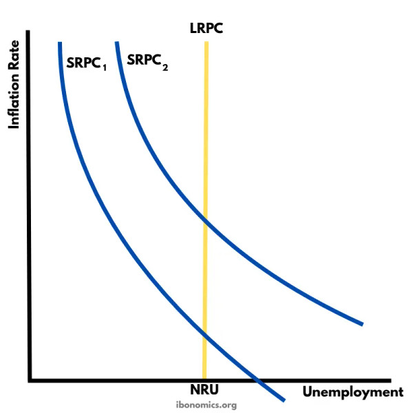
Short-Run and Long-Run Phillips Curves

The SRPC is downward sloping, showing an inverse relationship:

• Low unemployment → High inflation
• High unemployment → Low inflation

The economy is always operating somewhere along one of these short-run curves.

Why? Because changes in aggregate demand (AD) create this trade-off:

• Expansionary AD → higher output → lower unemployment → higher price level → higher inflation
• Contractionary AD → lower output → higher unemployment → lower inflation

So movements along the SRPC come from demand shocks.

The Long-Run Phillips Curve (LRPC)

In the long run, the Phillips Curve looks different.

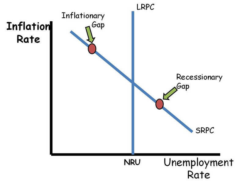
Long-Run Phillips Curve at the Natural Rate of Unemployment

The LRPC is vertical at the natural rate of unemployment (NRU).

Natural rate = frictional + structural unemployment.
It corresponds to full employment and the LRAS in the AD-AS model.

This means:

• There is no long-run trade-off between inflation and unemployment.
• Unemployment returns to the natural rate over time.

Policy can permanently change inflation.
It cannot permanently push unemployment below the natural rate.

2. Short-Run and Long-Run Equilibrium

Long-Run Equilibrium

Long-run equilibrium occurs where:

• SRPC intersects LRPC
• Unemployment = natural rate
• Inflation is stable

This matches the AD-AS model where AD, SRAS, and LRAS all intersect.

Inflationary and Recessionary Gaps

On the Phillips graph:

• Left of LRPC
  • Unemployment < natural rate
  • High inflation
  • Inflationary gap
• Right of LRPC
  • Unemployment > natural rate
  • Low inflation
  • Recessionary gap

Over time, expectations adjust:

• Inflationary gap → expected inflation rises → SRPC shifts right
• Recessionary gap → expected inflation falls → SRPC shifts left

The economy moves back to the natural rate.

This adjustment is why the long-run curve is vertical.

3. Demand Shocks and Movements Along the SRPC

Demand shocks cause movement along the existing SRPC.

Expansionary Demand Shock

Examples:

• Expansionary fiscal policy
• Expansionary monetary policy
• Increase in consumer confidence

Effects:

• Inflation rises
• Unemployment falls
• Movement up and left along SRPC

The late 1960s in the U.S. is a classic example. Expansionary policies reduced unemployment but led to rising inflation.

Contractionary Demand Shock

Examples:

• Higher taxes
• Reduced government spending
• Tight monetary policy

Effects:

• Inflation falls
• Unemployment rises
• Movement down and right along SRPC

If a question says “AD increases,” your brain should immediately think movement along SRPC, not a shift.

4. Supply Shocks and Shifts of the Curves

Supply shocks shift the SRPC itself.

Negative Supply Shock

A negative supply shock shifts the short-run Phillips curve to the right, meaning higher inflation at every level of unemployment.

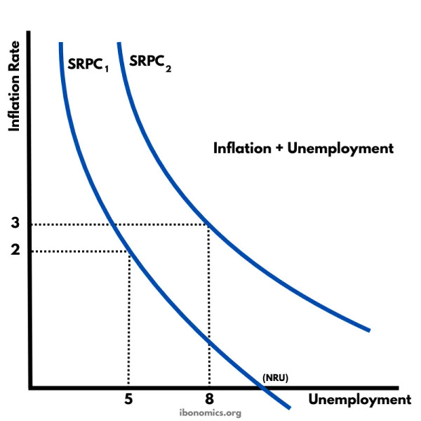
Rightward shift of the short-run Phillips curve after a negative supply shock

In the graph, the curve moves from SRPC₁ to SRPC₂, and the economy ends up with both higher inflation and higher unemployment.

Examples:

• 1970s oil price shocks
• Major increases in input costs
• Natural disasters

Effects:

• Higher inflation
• Higher unemployment
• SRPC shifts right

This creates stagflation. The U.S. in the 1970s experienced exactly this. High inflation and high unemployment at the same time broke the simple trade-off story.

Positive Supply Shock

A positive supply shock shifts the SRPC to the left, giving the economy lower inflation at every level of unemployment.

Examples:

• Technological improvements
• Decrease in input costs

Effects:

• Lower inflation
• Lower unemployment
• SRPC shifts left

5. Shifts of the Long-Run Phillips Curve

The LRPC shifts only when the natural rate changes.

Causes of changes in NRU:

• Labor market institutions (minimum wage laws, unions)
• Demographics
• Job matching efficiency (technology, education)
• Structural changes in the economy

If NRU increases → LRPC shifts right.
If NRU decreases → LRPC shifts left.

Paul Volcker’s disinflation in the early 1980s is a key historical example. The Federal Reserve reduced inflation, but unemployment temporarily rose as the economy adjusted back to the natural rate.