Topic 3.1 Notes – Aggregate Demand (AD)

1. What the Aggregate Demand Curve Is

Aggregate demand (AD) is the total spending on final goods and services at different price levels.

Here’s what the graph looks like:

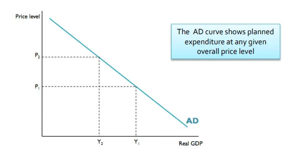
Aggregate demand (AD) curve

• Y-axis: Price Level
• X-axis: Real GDP (output)
• Shape: Downward sloping

As you move down the curve from a higher price level to a lower one, real GDP increases. The dashed lines in the graph highlight this inverse relationship between the price level and output.

Quick reminder. In micro, demand shows price of one good and quantity of that good. In macro, AD shows the overall price level and the total output of the economy. Instead of “quantity,” we use real GDP because GDP measures total production.

The Components of AD

Aggregate demand equals total spending:

$$AD = C + I + G + (X - M)$$

• C (Consumption): Household spending on goods and services
• I (Investment): Business spending on capital and new residential housing
• G (Government Spending): Government purchases of goods and services
• X − M (Net Exports): Exports minus imports

This connects back to GDP. On the spending side, GDP is calculated using this exact formula. AD simply shows how that total spending changes as the price level changes.

2. Why the AD Curve Slopes Downward

When the price level rises, the quantity of real GDP demanded falls. Three specific effects explain this.

1. Real Wealth Effect (Real Balances Effect)

Higher price level → money has less purchasing power → consumers feel poorer → C decreases.

Lower price level → purchasing power rises → C increases.

Think about high inflation in the 1970s. As prices climbed, households could afford less with the same income, so spending weakened.

2. Interest Rate Effect

Higher price level → people need more money for transactions → money demand rises → interest rates rise.

Higher interest rates → firms borrow less → Investment decreases.

Lower price level → lower interest rates → Investment increases.

This is what happened during the early 1980s when the Federal Reserve, led by Paul Volcker, pushed interest rates very high to fight inflation. Investment spending dropped sharply.

3. Exchange Rate Effect (Foreign Trade Effect)

Higher domestic price level → U.S. goods become more expensive relative to foreign goods → exports fall, imports rise → Net exports decrease → less spending on domestic output.

Lower domestic price level → U.S. goods become cheaper relative to foreign goods → exports rise, imports fall → Net exports increase.

All three effects together give AD its negative slope.

Important test detail:
A change in the price level causes a movement along AD, not a shift.

3. Movement Along AD vs. Shifts of AD

Movement Along the Curve

Only caused by a change in the price level.

Example: A drought in China causes inflation. That is a higher price level. Real GDP demanded falls. That’s a movement up along AD.

Students often confuse this with a shift. If inflation is the cause, stay on the same curve.

Shifts of the AD Curve

AD shifts when C, I, G, or NX changes for reasons other than the price level.

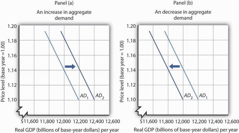
Right shift means more total spending.
Left shift means less total spending.

The left panel below shows an increase in aggregate demand, shifting the curve right from AD₁ to AD₂. The right panel shows a decrease in aggregate demand, shifting the curve left.

Changes in Consumption (C)

• Consumer confidence rises (example: stimulus payments in 2020) → AD shifts right.
• Tax cuts increase disposable income → AD right.
• Stock market crash reduces wealth → AD left.

Changes in Investment (I)

• Businesses expect higher profits → build more factories → AD right.
• Lower interest rates from Federal Reserve policy → AD right.
• Business pessimism during the 2008 financial crisis → AD left.

Changes in Government Spending (G)

• New Deal programs during the Great Depression → AD right.
• Government cuts military spending → AD left.

Changes in Net Exports (NX)

• Foreign economies boom → exports increase → AD right.
• Removal of a U.S. tariff increases imports → NX falls → AD left.
• Dollar appreciation reduces exports → AD left.

On multiple choice questions, they often describe a scenario like “consumer confidence soars in South Korea.” Your job is to identify the component and the direction. That is almost always what they’re testing.