Topic 3.4 Notes – Long-Run Aggregate Supply (LRAS)
1. What the Long Run Means in Macroeconomics
In macro, short run vs. long run is about price flexibility, not calendar time.
- Short run
- Some input prices, especially wages, are sticky.
- Firms respond to price level changes by changing output.
- Output can be above or below full employment.
- Long run
- All prices and wages are fully flexible.
- Contracts are renegotiated, expectations adjust.
- Workers demand higher wages if prices rise.
Because wages adjust fully in the long run:
- Real wages return to their original level.
- Firms’ costs return to normal.
- The economy returns to the natural rate of unemployment (NRU).
- There is no long-run trade-off between inflation and unemployment. (This connects to the vertical long-run Phillips Curve you saw earlier.)
Think of the 1970s stagflation. High inflation did not permanently reduce unemployment. Over time, the economy moved back to its natural rate.
In the AD-AS model, the short run explains recessions and booms. The long run shows where the economy settles after all adjustments.
2. What Long-Run Aggregate Supply Is
Long-Run Aggregate Supply (LRAS) is the economy’s maximum sustainable output.
It is:
- Also called full-employment output ( or )
- The level of Real GDP produced when:
- Labor is at the natural rate of unemployment
- Capital is fully utilized
- The economy operates at normal capacity
Why the LRAS Curve Is Vertical
Here’s the standard AD-AS graph with LRAS. Notice the vertical LRAS line at full-employment output (labeled Yf/Ye on this graph).
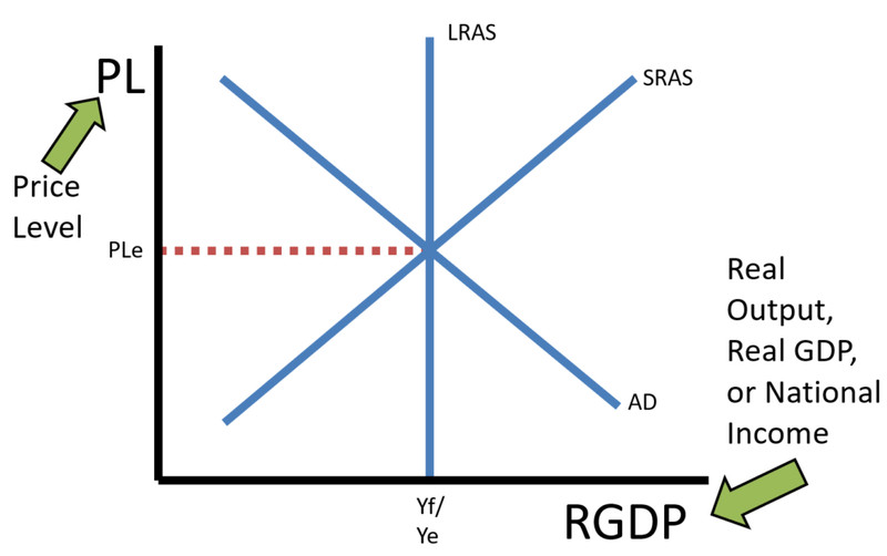
AD-AS model with vertical LRAS at full-employment output
LRAS is vertical at because:
- If the price level rises, wages rise proportionally in the long run.
- Real wages stay the same.
- Firms’ real costs stay the same.
- Firms have no reason to change output.
So in the long run:
- Changes in the price level do not change real GDP.
- Output depends on resources and productivity, not prices.
On this graph, you can shift AD to the right and raise the price level, but in the long run, real GDP returns to the vertical LRAS line.
3. LRAS and the Production Possibilities Curve
LRAS corresponds directly to the Production Possibilities Curve (PPC).
- Both represent maximum productive capacity.
- Both assume full employment of resources.
- Both shift when the economy’s capacity changes.
If the PPC shifts outward, LRAS shifts right. The outward movement of the frontier in the graph below represents economic growth and a higher level of potential output.
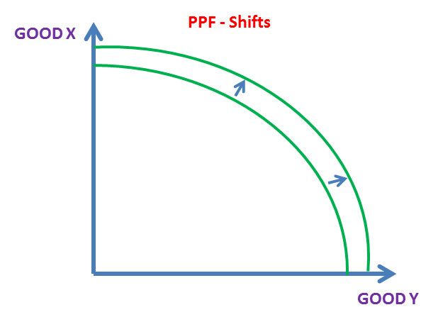
A rightward shift of LRAS means:
- Higher potential output
- Economic growth
Example anchors:
- Post-World War II U.S. expansion increased capital and labor → LRAS shifted right.
- The 1990s technology boom increased productivity → LRAS shifted right.
When you see “economic growth” in a question, think rightward shift of LRAS and outward shift of PPC.
4. What Shifts the LRAS Curve
LRAS shifts when productive capacity changes, not just current output.
A. Changes in the Quantity of Resources
- Labor
- Population growth or immigration → LRAS right
- Decrease in workforce → LRAS left
- Capital Stock
- More factories, machines, infrastructure → LRAS right
- War or natural disasters destroying capital → LRAS left
- Natural Resources
- Discovery of oil or fertile land → LRAS right
- Resource depletion → LRAS left
B. Changes in the Quality of Resources (Productivity)
- Human Capital
- Better education and training → more productive workers → LRAS right
- Deterioration of schools → LRAS left
- Technology
- Automation, AI, better logistics → higher productivity → LRAS right
Productivity growth is the core of long-run economic growth.
C. Policy Incentives
Government policies that increase:
- Labor force participation
- Investment in capital
- Research and development
Examples:
- Tax incentives for business investment
- Subsidies for education or job training
These increase potential output → LRAS shifts right.
5. LRAS vs. SRAS and Long-Run Adjustment
| Feature | SRAS | LRAS |
|---|---|---|
| Shape | Upward sloping | Vertical |
| Wages | Sticky | Fully flexible |
| Output | Can deviate from full employment | Fixed at full-employment level |
Long-Run Self-Correction
Recessionary gap:
- Output below LRAS
- High unemployment
- Wages fall
- SRAS shifts right
- Economy returns to
Inflationary gap:
- Output above LRAS
- Low unemployment
- Wages rise
- SRAS shifts left
- Economy returns to
This is why expansionary policy during a boom mainly causes inflation in the long run, not permanently higher output.
Key Takeaways
Short Run vs. Long Run
Short run has some fixed input prices; long run has fully flexible wages and prices.
Natural Rate of Unemployment
The unemployment rate that exists when the economy is producing at full employment.
Production Possibilities Curve (PPC) and LRAS
Both show an economy's maximum productive capacity, so outward PPC shifts match rightward LRAS shifts.
LRAS Shifters
Changes in resource quantity, resource quality, or policy that alter potential output.
Resource Quantity and LRAS
More labor, capital, or natural resources increase potential output; less shifts capacity downward.
Resource Quality and LRAS
Better education, skills, technology, or infrastructure raise productivity and increase potential output.
Policy and LRAS
Government incentives affecting work, investment, or productivity can increase or decrease potential output.
No Long-Run Inflation-Unemployment Trade-Off
With fully flexible wages and prices, inflation cannot permanently lower unemployment below its natural rate.
Long-Run Aggregate Supply (LRAS)
The economy's maximum sustainable real output when all resources are fully employed.
Long-Run Aggregate Supply Curve
A vertical curve at full-employment real GDP because wages and prices fully adjust.
LRAS Shifts
Changes in productive capacity shift the curve right with growth or left with decline.
Notes
Short Run vs. Long Run
Short run has some fixed input prices; long run has fully flexible wages and prices.
Natural Rate of Unemployment
The unemployment rate that exists when the economy is producing at full employment.
Production Possibilities Curve (PPC) and LRAS
Both show an economy's maximum productive capacity, so outward PPC shifts match rightward LRAS shifts.
LRAS Shifters
Changes in resource quantity, resource quality, or policy that alter potential output.
Resource Quantity and LRAS
More labor, capital, or natural resources increase potential output; less shifts capacity downward.
Resource Quality and LRAS
Better education, skills, technology, or infrastructure raise productivity and increase potential output.
Policy and LRAS
Government incentives affecting work, investment, or productivity can increase or decrease potential output.
No Long-Run Inflation-Unemployment Trade-Off
With fully flexible wages and prices, inflation cannot permanently lower unemployment below its natural rate.
Long-Run Aggregate Supply (LRAS)
The economy's maximum sustainable real output when all resources are fully employed.
Long-Run Aggregate Supply Curve
A vertical curve at full-employment real GDP because wages and prices fully adjust.
LRAS Shifts
Changes in productive capacity shift the curve right with growth or left with decline.
