Topic 3.2 Notes – Multipliers
1. The Multiplier Effect
A multiplier means an initial change in autonomous spending causes a larger overall change in real GDP.
In the AD-AS model, this shows up as a shift of the aggregate demand (AD) curve that is bigger than the original spending change.
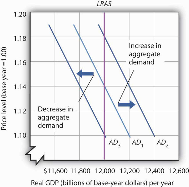
Shifts in aggregate demand in the AD-AS model
A rightward shift of AD, like the move from AD3 to AD2 in the graph, represents an increase in spending. The multiplier explains why that shift can be larger than the initial change in autonomous spending.
Why does this happen?
Because one person’s spending becomes another person’s income.
How the spending chain works
- The government, firms, or foreigners increase spending (for example, higher government spending, more investment, or more exports).
- That spending becomes income for households.
- Households spend part of that new income.
- That new spending becomes income for someone else.
- The cycle repeats, getting smaller each round because some income is saved.
The process continues until leakages, mainly saving (and in the real world also taxes and imports), shrink the rounds to almost zero.
This logic is straight from Keynesian economics. It explains why large spending programs like the New Deal during the Great Depression, the 2008 financial crisis stimulus, and COVID recession relief packages were expected to boost GDP by more than the initial dollars spent.
Key idea:
A 1-dollar increase in autonomous spending leads to a greater than 1-dollar increase in real GDP.
2. Marginal Propensity to Consume and Save
The size of the multiplier depends entirely on two numbers.
Marginal Propensity to Consume (MPC)
The MPC is the fraction of an additional dollar of disposable income that households spend.
If disposable income rises by 200 dollars and consumption rises by 150 dollars, then
.
That means households spend 75 cents of each extra dollar.
Marginal Propensity to Save (MPS)
The MPS is the fraction of additional disposable income that households save.
If savings rise by 50 dollars when income rises by 200 dollars, then
.
The key relationship
Every extra dollar is either spent or saved.
- Higher MPC → larger multiplier
- Higher MPS → smaller multiplier
On tests, you’re often given MPC and expected to find MPS using
. Don’t skip that step.
3. The Expenditure Multiplier
The expenditure multiplier measures the total change in GDP from a change in autonomous spending.
Applies to:
- Government spending (G)
- Investment (I)
- Autonomous consumption
- Net exports (X − M)
Formula
or
Calculating the change in GDP
Suppose:
- MPC = 0.8
- Government increases spending by 40 dollars
First, find MPS:
Multiplier:
Change in GDP:
Real GDP increases by 200 dollars.
Properties you should remember:
- Always positive
- Always greater than 1
- Directly shifts AD
- Works in reverse too. A spending cut reduces GDP by a multiplied amount.
4. The Tax Multiplier
The tax multiplier measures the total change in GDP from a change in taxes.
Taxes work differently because they change disposable income, not direct spending.
If taxes fall by 100 dollars and MPC is 0.8, households only spend 80 dollars of it. That smaller first-round effect makes the total impact smaller than with direct spending.
Formula
The negative sign matters.
Example
If:
- MPC = 0.75
- Taxes increase by 20 dollars
First, find MPS:
Tax multiplier:
Change in GDP:
GDP falls by 60 dollars.
Important patterns:
- Always negative
- Smaller in absolute value than the spending multiplier
- Tax increase → GDP decreases
- Tax decrease → GDP increases
5. Spending vs Tax Multipliers
| Spending Multiplier | Tax Multiplier | |
|---|---|---|
| Formula | ||
| Sign | Positive | Negative |
| Size | Larger | Smaller (absolute value) |
| Impact on AD | Direct | Indirect (through income) |
If policymakers want the biggest GDP impact per dollar, direct government spending is more powerful than tax changes.
Both multipliers explain how fiscal policy shifts AD in the AD-AS model. The size of that shift depends completely on MPC and MPS.
Key Takeaways
Multiplier Effect
An initial change in spending causes a larger overall change in real GDP.
Why The Tax Multiplier Is Smaller Than The Expenditure Multiplier
Tax changes affect spending only through disposable income, so only the consumed portion is multiplied.
Autonomous Expenditures
Spending changes that occur independently of current real GDP and start the multiplier process.
Marginal Propensity To Consume (MPC) And Marginal Propensity To Save (MPS)
They are the fractions of each additional disposable income dollar spent and saved.
Calculating MPC And MPS
They equal changes in consumption and saving over disposable income, and together sum to one.
Expenditure Multiplier
It equals 1 divided by MPS, showing total real GDP change from autonomous spending.
Tax Multiplier
It equals negative MPC divided by MPS, showing real GDP change from taxes.
Calculating Change In Real GDP With Multipliers
Multiply the initial change by the multiplier; spending and GDP match, while taxes move oppositely.
Notes
Multiplier Effect
An initial change in spending causes a larger overall change in real GDP.
Why The Tax Multiplier Is Smaller Than The Expenditure Multiplier
Tax changes affect spending only through disposable income, so only the consumed portion is multiplied.
Autonomous Expenditures
Spending changes that occur independently of current real GDP and start the multiplier process.
Marginal Propensity To Consume (MPC) And Marginal Propensity To Save (MPS)
They are the fractions of each additional disposable income dollar spent and saved.
Calculating MPC And MPS
They equal changes in consumption and saving over disposable income, and together sum to one.
Expenditure Multiplier
It equals 1 divided by MPS, showing total real GDP change from autonomous spending.
Tax Multiplier
It equals negative MPC divided by MPS, showing real GDP change from taxes.
Calculating Change In Real GDP With Multipliers
Multiply the initial change by the multiplier; spending and GDP match, while taxes move oppositely.
