Topic 3.5 Notes – Equilibrium in the Aggregate Demand–Aggregate Supply (AD–AS) Model

1. Short-Run Equilibrium in the AD-AS Model

In the short run, equilibrium happens where Aggregate Demand (AD) intersects Short-Run Aggregate Supply (SRAS).

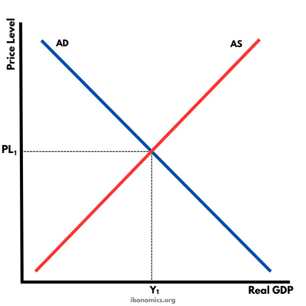
Short-run AD-AS equilibrium

In the graph, the downward-sloping AD curve intersects the upward-sloping AS curve (representing SRAS) at equilibrium output Y₁ and price level PL₁.

At this intersection:

• Quantity of real GDP demanded = quantity supplied
• The economy settles at a specific price level (PL) and real GDP (Y)
• There’s no pressure for output or prices to change

This works just like micro supply and demand, except instead of one product, we’re talking about total output in the entire economy.

What if the price level isn’t at equilibrium?

• If price level is above equilibrium
  • SRAS > AD → surplus of output
  • Unsold goods pile up → firms lower prices
  • Economy moves back toward equilibrium
• If price level is below equilibrium
  • AD > SRAS → shortage of output
  • Firms raise prices
  • Economy moves back toward equilibrium

On tests, when you’re asked for short-run equilibrium output and price level, you mark the intersection of AD and SRAS, even if it’s not at full employment.

2. Long-Run Equilibrium and Full Employment

Long-run equilibrium adds one more curve: Long-Run Aggregate Supply (LRAS).

LRAS is vertical at potential GDP, which represents the full-employment level of real output.

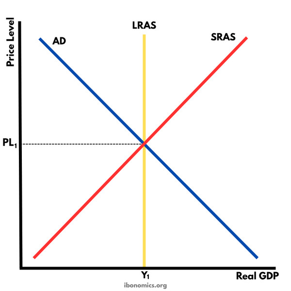
Long-run equilibrium in the AD-AS model

In the graph above, AD and SRAS intersect exactly on the vertical LRAS line at output Y₁ and price level PL₁.

Long-run equilibrium occurs when:

• AD intersects SRAS
• And that intersection lies on LRAS

At this point:

• Real GDP = potential GDP
• Unemployment = natural rate (about 4-6%)
• No cyclical unemployment
• No inflationary or recessionary gap

This is the economy operating at its sustainable capacity. Think of the late 1990s tech boom when output was near full employment before inflation pressures started building.

3. Output Gaps

Short-run equilibrium doesn’t have to occur at potential GDP. That’s where output gaps come in.

There are two types.

Recessionary Gap (Negative Output Gap)

This happens when short-run equilibrium is left of LRAS.

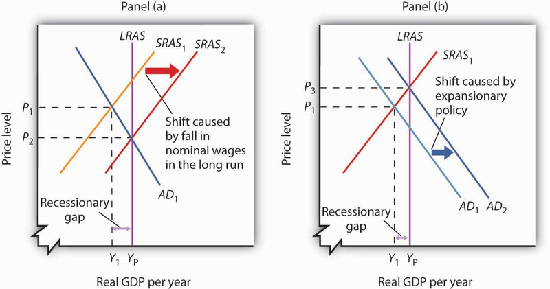
Recessionary gap in the AD-AS model

In the diagrams above, focus on the equilibrium where output (Y₁) is to the left of potential output (Y_P). The horizontal distance between them is the recessionary gap.

What it means:

• Real GDP < potential GDP
• High cyclical unemployment
• Weak demand
• Downward pressure on wages and production costs

Historical anchor:
During the Great Depression and again in the 2008-2009 Great Recession, the U.S. economy operated far below potential GDP. High unemployment signaled a large recessionary gap.

Inflationary Gap (Positive Output Gap)

This happens when short-run equilibrium is right of LRAS.

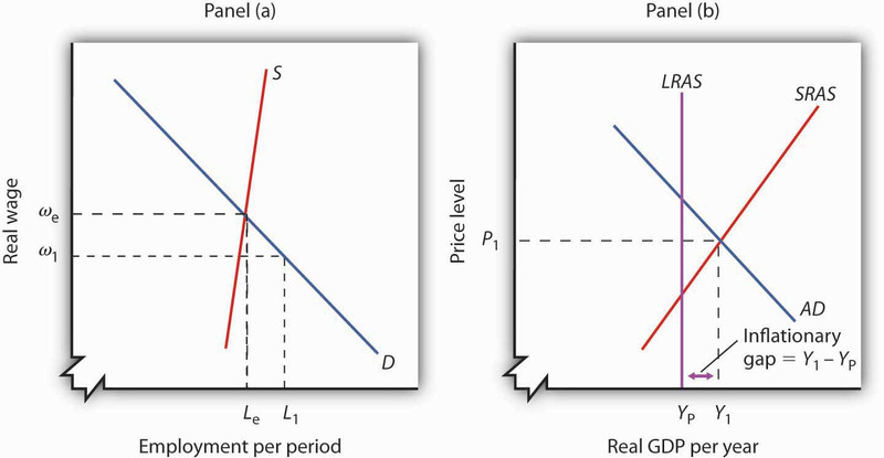
Inflationary gap in the AD-AS model

Here, equilibrium output (Y₁) is to the right of potential output (Y_P). The distance between them represents the inflationary gap.

What it means:

• Real GDP > potential GDP
• Unemployment below natural rate
• Strong demand
• Upward pressure on wages and prices

Historical anchor:
In 2006, before the housing crash, low unemployment and heavy spending pushed the economy above potential. That overheating created inflationary pressure.

This is also what policymakers worried about in the late 1960s before the high inflation of the 1970s.

How the Economy Self-Corrects

In the basic AD-AS model, the economy moves back to long-run equilibrium through wage adjustments.

If there’s a recessionary gap:

1. High unemployment → excess labor supply
2. Wages fall
3. Production costs fall
4. SRAS shifts right
5. Output returns to potential GDP

If there’s an inflationary gap:

1. Labor shortages
2. Wages rise
3. Production costs rise
4. SRAS shifts left
5. Output falls back to potential GDP

In both cases, real GDP returns to potential, but the price level changes permanently.

Later topics bring in fiscal policy and the Federal Reserve’s monetary policy responses. For now, the key is understanding how equilibrium works before policy enters the picture.