Topic 1.2 Notes – Displacement, Velocity, and Acceleration

1. Position and Displacement

The object model

In mechanics, we usually treat objects as point particles. That means:

• The object is modeled as a single point in space.
• We ignore size, shape, and internal structure.
• All mass (and charge, if relevant) is treated as located at that point.

This works when the object’s size is tiny compared to the distances involved. A car driving 200 m can be treated as a point. A rotating disk in a torque problem cannot.

Once we do that, motion becomes tracking position as a function of time.

Position

Position tells you where the object is relative to an origin you choose.

• In 1D:
  $x(t)$
• In 2D or 3D:
  $$\vec{r}(t) = x(t)\hat{i} + y(t)\hat{j} + z(t)\hat{k}$$

That vector notation matters. Direction is built in.

Displacement

Displacement is the change in position.

In 1D:
$$\Delta x = x - x_{0}$$

In vector form:
$$\Delta \vec{r} = \vec{r} - \vec{r}_{0}$$

Key ideas:

• It is a vector.
• It depends only on initial and final positions.
• If you return to where you started, displacement is zero, even if you traveled 5 km.

In multiple dimensions, subtract components separately:
$$\Delta x = x - x_{0}, \quad \Delta y = y - y_{0}$$

On free response, students often accidentally use distance instead of displacement. If direction matters, you need the vector.

2. Average Velocity and Average Acceleration

Average quantities describe motion over a finite time interval. They only care about the start and end.

Average velocity

$$\vec{v}_{\text{avg}} = \frac{\Delta \vec{r}}{\Delta t}$$

• Direction matches displacement.
• Can be zero if you end where you started.
• Not the same as average speed (which uses total distance).

If someone walks 10 m right, then 10 m left in 4 s:

• $\Delta x = 0$
• $v_{\text{avg}} = 0$

But the average speed is $20/4 = 5 \,\text{m/s}$.

Average acceleration

$$\vec{a}_{\text{avg}} = \frac{\Delta \vec{v}}{\Delta t}$$

Acceleration happens whenever velocity changes, meaning:

• Speed changes.
• Direction changes.
• Or both.

A car turning at constant speed in a circle is accelerating because its velocity vector keeps changing direction. That’s a favorite conceptual trap on multiple choice.

As $\Delta t$ gets very small, average values approach instantaneous ones. That’s the bridge to calculus.

3. Instantaneous Velocity and Acceleration

Instantaneous values describe motion at a single moment. They come from limits.

Instantaneous velocity

$$\vec{v} = \frac{d\vec{r}}{dt} \quad \text{(in 1D: } v_{x} = \frac{dx}{dt}\text{)}$$

Two ways to think about it:

• Mathematically: derivative of position.
• Graphically: slope of the position vs. time graph.

The stacked graphs below show all three relationships for one motion. The top curve is position vs. time, the middle line is velocity vs. time, and the bottom horizontal line is acceleration vs. time.

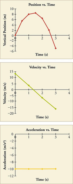
Position, velocity, and acceleration vs. time for one object

The steeper the position graph at a point, the larger the velocity there. Notice how the position graph reaches a peak when the velocity graph crosses zero.

Instantaneous acceleration

$$\vec{a} = \frac{d\vec{v}}{dt} \quad \text{(in 1D: } a_{x} = \frac{d^{2} x}{dt^{2}}\text{)}$$

So acceleration is:

• Slope of the velocity vs. time graph.
• Second derivative of position.

In the figure, velocity decreases linearly with time, so the acceleration is constant and negative, shown by the flat line on the bottom graph.

Instantaneous as a limit

Conceptually:
$$\frac{\Delta x}{\Delta t} \to \frac{dx}{dt} \quad \text{as } \Delta t \to 0$$

That limit idea is what makes Physics C calculus-based. On FRQs, when they say “determine the velocity at time $t$,” they expect a derivative.

4. Connecting Position, Velocity, and Acceleration Functions

In this course, you’re often given one function and asked for the others.

From position down to acceleration

If $x(t)$ is given:

1. Differentiate once → $v(t) = \dfrac{dx}{dt}$
2. Differentiate again → $a(t) = \dfrac{d^{2} x}{dt^{2}}$

Example:
If $x(t) = 4t^{3} - 2t$

$$v(t) = 12t^{2} - 2$$

$$a(t) = 24t$$

Plug in a time if they want a value at a specific instant.

From acceleration or velocity back up

Integrals give net change:

$$\Delta v = \int_{t_{1}}^{t_{2}} a(t)\,dt$$ $$\Delta x = \int_{t_{1}}^{t_{2}} v(t)\,dt$$

Graphically:

• Area under $v(t)$ → displacement.
• Area under $a(t)$ → change in velocity.

If you integrate an expression (indefinite integral), you must include a constant. That constant comes from an initial condition like $x(0) = 3$.

Students lose points when they forget that constant.

The chain to memorize

Position → derivative → velocity → derivative → acceleration
Acceleration → integral → velocity → integral → position

That structure shows up everywhere in mechanics.