Topic 5.5 Notes – Rotational Equilibrium and Newton’s First Law in Rotational Form
1. Rotational Equilibrium and Constant Angular Velocity
An object is in rotational equilibrium when its angular velocity is constant.
That includes two situations:
- (not rotating)
- (spinning steadily)
The condition for this is:
If the net torque is zero, then:
This is the rotational version of Newton’s First Law.
- No net force → no change in linear motion
- No net torque → no change in rotational motion
If torques are unbalanced, the object must have angular acceleration. Its rotation is speeding up or slowing down.
AP Physics 1 keeps this simple:
- Single, fixed axis of rotation
- No multiple-plane rotation analysis
2. Translational vs Rotational Equilibrium
These are separate conditions. Always check them independently.
Translational Equilibrium
- No linear acceleration
- Object could be at rest or moving at constant velocity
Rotational Equilibrium
- No angular acceleration
- Object could be stationary or spinning at constant speed
Here’s how the linear and rotational ideas line up:
| Linear Motion | Rotational Motion |
|---|---|
| Force | Torque |
| Mass | Moment of inertia |
| Acceleration | Angular acceleration |
An object can have one without the other.
- A spinning ball tossed through the air has (gravity) but about its center of mass (gravity acts through the CM), so it accelerates linearly while spinning at constant .
- A sliding block can have but still experience a net torque about some chosen axis.
That second situation shows up in multiple-choice questions where they change the axis and try to trick you.
3. Torque and How to Calculate Net Torque
What torque actually is
Torque measures how strongly a force causes rotation about an axis.
- is distance from axis to point of force
- is angle between and
You’ll often use:
The lever arm is the perpendicular distance from the axis to the force’s line of action.
The diagram below shows a rod pivoted at the left end with the same force applied in different ways.
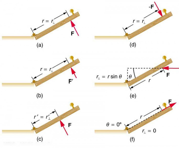
Notice how the perpendicular distance from the pivot changes depending on the angle. When the force is perpendicular to the rod, the torque is largest. When the force points along the rod toward the pivot, the lever arm is zero and the torque is zero.
Signs
- Counterclockwise → positive
- Clockwise → negative
Pick one convention and stay consistent.
Net torque
Add torques algebraically, including signs:
- → rotational equilibrium
- → angular acceleration
Choosing the axis strategically helps. If you choose the pivot, forces applied there produce zero torque, which simplifies your equation. That’s a favorite move on ladder and beam problems.
4. Free-Body Diagrams for Rotational Systems
Every rotational problem starts with a free-body diagram.
Include:
- All external forces
- Correct directions
- Points of application
Here’s a typical example structure for a beam fixed to a wall and supporting a load:
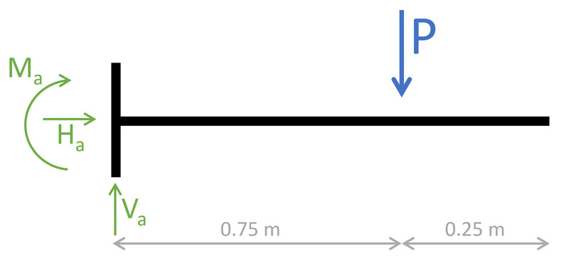
Free-body diagram of a cantilever beam with applied load and wall reactions
The downward force on the beam is shown, along with the reaction forces at the wall and the reaction moment that prevents rotation. That reaction moment is what keeps the beam from spinning clockwise under the load.
For full equilibrium problems, you usually need:
Three equations. Three unknowns. Solve systematically.
On FRQs, students often forget one of the force equations and lose easy points.
5. Static Friction in Rotational Equilibrium
Static friction shows up constantly in rotational equilibrium.
It is adjustable:
It matches whatever force is needed up to its maximum.
Key ideas:
- Acts parallel to surfaces
- Direction prevents slipping
- Only equals at the verge of motion
In ladder-style problems:
- Static friction provides a torque.
- If required friction exceeds , equilibrium fails and slipping begins.
When solving:
- Draw FBD.
- Apply force equilibrium.
- Apply torque equilibrium about a smart axis.
- Only substitute if the problem says “about to slip” or asks for a maximum.
