Topic 1.3 Notes – Rates of Change in Linear and Quadratic Functions

Average rate of change

For a function $f$, the average rate of change on $[a,b]$ is

$$\frac{f(b)-f(a)}{b-a}$$

This is output change divided by input change. It works on any interval, and the interval does not have to start at 0.

On a graph, this is the slope of the secant line through $(a,f(a))$ and $(b,f(b))$.

A quick example with $f(x)=x^2$ on $[1,3]$:

$$\frac{f(3)-f(1)}{3-1}=\frac{9-1}{2}=4$$

That means the output increased by an average of 4 units for each 1 unit of input over that interval.

This also works for sequences. If a sequence is $u_n$, then from index $i$ to $j$,

$$\frac{u_j-u_i}{j-i}$$

For consecutive terms, that becomes $u_{n+1}-u_n$, which is the first difference.

From different representations:

• Table: use the two rows with inputs $a$ and $b$
• Graph: read or estimate the endpoint coordinates
• Context: include units, like “feet per second” or “dollars per hour”

Rate patterns for linear and quadratic functions

This is the big comparison you need to know.

Linear functions

If $L(x)=mx+c$, then the average rate of change over any interval is always $m$.

• Every secant line has the same slope as the graph itself
• Over equal-length intervals, the average rates stay constant
• The change in those average rates is $0$

Example with $L(x)=2x-5$:

$$\frac{L(7)-L(1)}{7-1}=\frac{9-(-3)}{6}=2$$

You would get 2 on every interval. A constant function is the special case $m=0$.

Quadratic functions

If $q(x)=Ax^2+Bx+C$, the average rate depends on the interval.

Over $[a,b]$,

$$\frac{q(b)-q(a)}{b-a}=A(a+b)+B$$

For a fixed interval length $h$,

$$R_h(x)=\frac{q(x+h)-q(x)}{h}=2Ax+Ah+B$$

That matters because $R_h(x)$ is linear in $x$. So for equal-length intervals, the average rates of change follow a linear pattern.

• consecutive equal-length intervals change by $2Ah$
• per 1-unit increase in interval location, the rates change by $2A$
• for unit intervals, consecutive average rates differ by $2A$

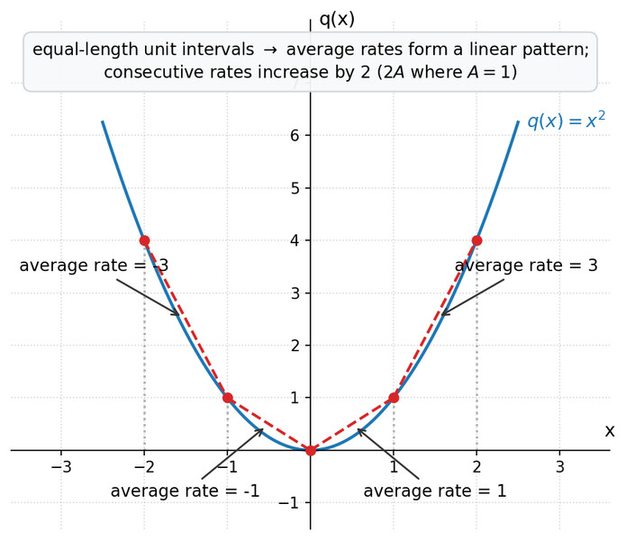
In the graph below, the unit-interval average rates for $q(x)=x^2$ are $-3$, $-1$, $1$, and $3$. They increase by 2 each time, which matches $2A$ when $A=1$.

How to find and compare rates

When you calculate one, the moves are always the same:

1. Pick the interval endpoints
2. Find the two outputs
3. Subtract outputs
4. Subtract inputs
5. Divide
6. Interpret the sign and units

For sequences, if the index step is 1, use the first difference.

If table inputs are equally spaced by $h$, then

$$\text{average rate}=\frac{\text{first output difference}}{h}$$

When comparing several intervals, check that they have the same length before deciding whether the pattern looks linear or quadratic.

Keep these three ideas separate, because AP questions love mixing them up:

• the average rate
• the change from one average rate to the next
• the rate at which the average rates are changing

Concavity and what changing rates mean

Concavity is about whether the rates are increasing or decreasing.

• If average rates over equal small intervals are increasing, the graph is concave up
• If they are decreasing, the graph is concave down

For quadratics, the sign of $A$ tells you everything:

• $A>0$ $\rightarrow$ concave up
• $A<0$ $\rightarrow$ concave down

Linear functions have constant average rates, so their change in rate is zero.

One common trap: a function can be decreasing while concave up, or increasing while concave down. Concavity is not about whether the function values rise or fall. It’s about what the rates are doing.

Common mistakes and fast checks

• Using $f(b)-f(a)$ alone as the rate. You still need to divide by $b-a$.
• Mixing up a secant slope with a tangent-line idea. This topic is interval-based.
• Comparing intervals of different lengths as if the pattern should still match.
• Saying quadratics have constant average rate. They do not. Their changes in average rate are constant.
• Saying a zero average rate means the function stayed constant. It only means the endpoints have equal outputs.
• Assuming bigger $y$-values mean bigger rates.
• Forgetting units, especially for the “rate of the rates” like meters per second per second.