Topic 2.6 Notes – Competing Function Model Validation

Linear vs quadratic vs exponential models

A lot of data sets are tricky because they have slight curvature. Over a short interval, the graph might look almost straight, even if a quadratic or exponential model fits too.

Here’s the pattern you look for, especially when the $x$-values are equally spaced:

• Linear $y=mx+b$
  • has about constant first differences
  • means the output changes by about the same amount each step
• Quadratic $y=ax^2+bx+c$
  • has about constant second differences
  • means the rate of change is changing steadily
• Exponential $y=ab^x$
  • has about constant ratios
  • means the output changes by about the same factor or percent each step

This quick visual review can help you keep the three graph shapes straight as you compare them.

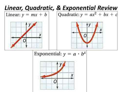
Linear, quadratic, and exponential parent shapes

If inputs are not equally spaced, first differences and ratios are less helpful. Then you compare change over equal-length intervals if possible, and rely more on the graph and regression results.

One caution that shows up on tests a lot: these numerical clues suggest a model family, but they do not prove it.

Building and comparing the candidate models

You usually compare all three candidates from the same data set.

1. Look at the table or scatterplot.
   • Is the change roughly constant, steadily bending, or changing by percent?
2. Build each model.
   • Linear from regression, or from two exact points
   • Quadratic from regression, or from three exact points
   • Exponential from regression, or from two suitable exact points
3. Compare both the fit and the context.

Technology forms you need to recognize are

$$y=ax+b$$

$$y=ax^2+bx+c$$

$$y=ab^x$$

Be careful with calculator letters. In linear regression, $a$ might be slope. In quadratic regression, $a$ is the coefficient of $x^2$. Same letter, different meaning.

Common AP-style situations here:

• Linear, quadratic, and exponential models from the same data set
• Data with a slightly changing rate of change that could plausibly fit more than one family

Residuals and what their signs mean

A residual is

$$r=\text{actual}-\text{predicted}=y-\hat y$$

It is the signed vertical distance from the data point to the model.

• $r>0$ means the actual point is above the model.
  • The model underestimates.
• $r<0$ means the actual point is below the model.
  • The model overestimates.
• $r=0$ means an exact prediction.

The absolute error is $|r|$. That tells you the size of the miss, but not the direction.

A very common trap is reversing the subtraction. If the point is above the graph, the model predicted too low, so that is an underestimate.

Over an interval:

• mostly positive residuals $\rightarrow$ model tends to underestimate
• mostly negative residuals $\rightarrow$ model tends to overestimate

Sometimes one direction is better in context. Overestimating supply needs may be safer. Underestimating capacity may be safer.

Residual plots and model validation

A residual plot uses original $x$-values on the horizontal axis and residuals on the vertical axis.

The line $r=0$ means perfect prediction.

A model is considered appropriate when residuals are scattered around zero with no visible pattern.

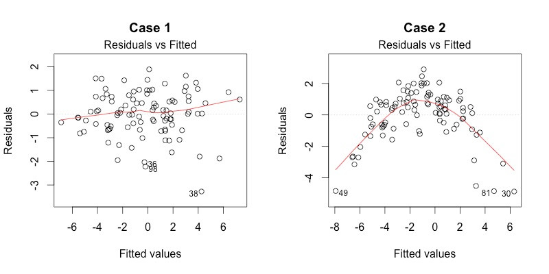
Residual plots with and without a pattern

In the image, focus on the overall shape of the residuals. The left plot shows the kind of random scatter you want. The right plot shows a curved pattern, which suggests the model is missing structure in the data.

Patterns that mean the model should be questioned:

• U-shape or curved pattern
• inverted U-shape
• upward or downward trend
• long runs of mostly positive or mostly negative residuals
• wave-like pattern

This matters more than a “close-looking” scatterplot fit because two models can look similar on the original graph, but residuals expose hidden structure.

Good justification language:

• The model is appropriate because its residual plot shows no discernible pattern.
• The competing model is less appropriate because its residual plot shows a systematic pattern.

Choosing the best model in context

The best model is not just the one with small errors. You also need a model whose behavior makes sense.

• Linear fits constant additive change.
• Quadratic fits a turning point or steadily changing rate.
• Exponential fits constant percent/proportional change and usually situations that stay positive.

Also keep interpolation vs extrapolation in mind. A model can work well inside the data range and still give unrealistic predictions outside it.

Context checks worth mentioning in conclusions:

• Can outputs be negative?
• Can the quantity reverse direction?
• Is constant difference or constant ratio more realistic?
• Are long-term predictions believable?

Common mistakes:

• choosing from the scatterplot without checking residuals
• treating a patternless residual plot as proof the model is “true”
• ignoring whether overestimates or underestimates are acceptable