Topic 2.15 Notes – Semi-log Plots

Reading exponential data on a log scale

A semi-log plot uses a linear horizontal axis and a logarithmic vertical axis. On the $x$-axis, equal spacing means equal addition. On the $y$-axis, equal spacing means equal multiplication.

On a base-$n$ log scale, the values $1,\ n,\ n^2,\ n^3$ are equally spaced because their logs are $0,1,2,3$.

• Base 10 example: $1,10,100,1000$ are equally spaced
• Base 2 example: $1,2,4,8$ are equally spaced

That is the whole visual idea. A constant vertical rise means a constant factor, not a constant difference.

In the base-10 graph below, those equal vertical steps line up with $1,10,100,$ and $1000$, so the exponential $y=10^x$ appears as a straight line.

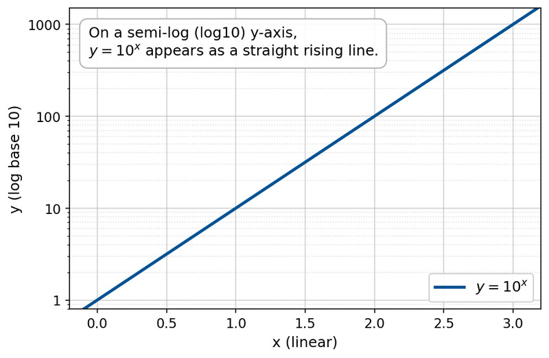
Semi-log plot of $y=10^x$

One restriction matters a lot. Only positive $y$-values can go on a logarithmic axis. You cannot plot $y=0$ or negative outputs there.

Why this helps with exponentials comes from logs:

$$\log_n y=(\log_n b)x+\log_n a$$

for an exponential model

$$y=ab^x$$

So taking the log of the outputs turns an exponential relationship into a linear one. A semi-log graph does that visually.

Recognizing When an Exponential Model Fits

Here’s the comparison teachers love to test:

• Straight on an ordinary graph $\Rightarrow$ linear in the original variables
• Straight on a semi-log graph $\Rightarrow$ exponential in the original variables

If the semi-log graph bends in a clear pattern, then a simple $y=ab^x$ model does not fit.

Real data will almost never land perfectly on one line. What you want is approximate linearity.

A subtle but important case shows up when only the large-$x$ values look linear on the semi-log graph. That points to a transformed exponential, often something like

$$y=ab^x+k$$

The key conclusion is this: eventual linearity supports a transformed exponential model, not automatically a pure unshifted exponential.

That is one advantage of semi-log plots. You can spot exponential-type behavior without first guessing and subtracting a constant shift.

Building the Linearization and Recovering the Exponential Model

If you begin with

$$y=ab^x$$

then the linearized form is

$$\log_n y=x\log_n b+\log_n a$$

This means:

• slope on the linearized graph is $\log_n b$, not $b$
• intercept on the linearized graph is $\log_n a$, not $a$

If the transformed line is

$$\log_n y=mx+c$$

then recover the exponential model with

$$b=n^m \qquad a=n^c$$

so

$$y=ab^x=(n^c)(n^m)^x$$

There are two equivalent ways to view the same thing:

• plot $(x,\log_n y)$ on ordinary axes
• plot $(x,y)$ on a graph with a logarithmic $y$-axis

Be careful with intercepts. On the transformed graph, the intercept is $\log_n a$. On the semi-log graph, the point at $x=0$ has original $y$-value $a$.

How to Construct and Use a Semi-log Model

A clean process looks like this:

1. Check that all outputs are positive.
2. Choose a log base $n>1$, often $10$, $2$, or $e$.
3. Graph the data on a semi-log plot or compute $(x,\log_n y)$.
4. Decide whether the transformed data are approximately linear.
5. Use linear methods to find $m$ and $c$.
6. Write $\log_n y=mx+c$.
7. Convert back with $a=n^c$ and $b=n^m$.

Example: if $\log_2 y=-x+3$, then

• $m=-1$, so $b=2^{-1}=\frac12$
• $c=3$, so $a=2^3=8$

Model:

$$y=8\left(\frac12\right)^x$$

On a base-2 semi-log plot, that model appears as a straight decreasing line, which is exactly what you want to see after linearizing exponential decay.

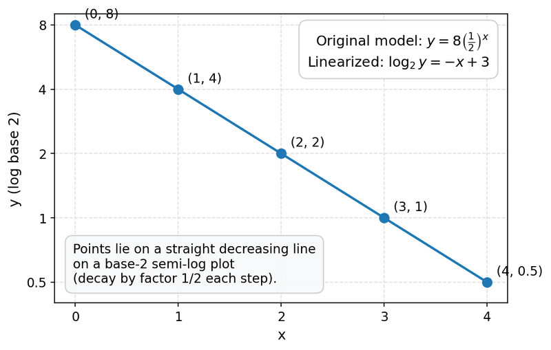
Base-2 semi-log graph of $y=8\left(\frac12\right)^x$

Interpret the slope sign carefully:

• $m>0 \Rightarrow b>1$ growth
• $m<0 \Rightarrow 0<b<1$ decay
• $m=0 \Rightarrow b=1$, which is constant and not exponential by the course definition

Common Mistakes and Fast Checks

The most common mistakes are quick to say and expensive on a test.

• Reading the slope as $b$ instead of $\log_n b$
• Reading the intercept as $a$ instead of $\log_n a$
• Forgetting to exponentiate to get back $a$ and $b$
• Calling a straight semi-log graph linear in the original variables
• Trying to place $0$ or negative outputs on the log axis
• Thinking a different log base changes whether the data linearizes

Changing base changes the numerical slope and intercept, but exponential data still appears linear.