Topic 1.4 Notes – Polynomial Functions and Rates of Change

What Polynomial Functions Are

A polynomial function can be written as

$$p(x)=a_nx^n+a_{n-1}x^{n-1}+\cdots+a_1x+a_0$$

where $n$ is a nonnegative integer, $a_n\neq 0$, and the coefficients are real numbers.

A few terms here matter a lot:

• Degree = the highest exponent, so the degree is $n$
• Leading term = the term with the highest power, $a_nx^n$
• Leading coefficient = the coefficient of that term, $a_n$

A nonzero constant like $p(x)=4$ is still a polynomial. Its degree is 0.
The zero polynomial is also a polynomial, but its degree is undefined.

A polynomial does not have to be expanded. For example, $(x-2)^2(x+5)$ still counts because it’s equivalent to polynomial form.

Usually, the domain is all real numbers unless the problem restricts it. Graphically, polynomials are:

• continuous so there are no breaks, holes, or jumps
• smooth so there are no corners or vertical asymptotes

One rate idea drives the whole topic. The average rate of change on $[a,b]$ is

$$\frac{p(b)-p(a)}{b-a}$$

Its sign tells you whether outputs are going up or down over that interval.

Increasing, Decreasing, and Extrema

A polynomial is increasing on an interval when bigger $x$-values give bigger $y$-values. It is decreasing when bigger $x$-values give smaller $y$-values.

From rates of change:

1. Positive average rates suggest increasing behavior.
2. Negative average rates suggest decreasing behavior.
3. A switch from positive nearby rates to negative nearby rates suggests a local maximum.
4. A switch from negative nearby rates to positive nearby rates suggests a local minimum.

Be careful with tables. You must compare rates, not just output differences, unless the input intervals are equal.

A local maximum happens where the graph changes from increasing to decreasing.
A local minimum happens where it changes from decreasing to increasing.

Keep these separate:

• $c$ is the input
• $p(c)$ is the maximum or minimum output
• $(c,p(c))$ is the point

Local and relative mean the same thing.

A global maximum is the greatest output on the whole domain. A global minimum is the least output on the whole domain. A local extremum does not have to be global, and the same global value can happen at more than one input.

If the domain is restricted, an included endpoint can be a local or global extremum. An excluded endpoint cannot.

For even degree polynomials:

• positive leading coefficient $\rightarrow$ guaranteed global minimum
• negative leading coefficient $\rightarrow$ guaranteed global maximum

For quadratics, that global extremum is at the vertex.

Real Zeros and the Required Extremum Between Them

A real zero is an input $a$ such that $p(a)=0$. On the graph, that gives an $x$-intercept $(a,0)$.

Between every two distinct real zeros of a nonconstant polynomial, there is at least one local maximum or minimum. That is a guarantee of at least one, not exactly one.

A zero does not automatically mean extremum.

Example:

$$p(x)=x^4-6x^2=x^2(x^2-6)$$

Its distinct real zeros are $-\sqrt6,\ 0,\ \sqrt6$. Its local minima are at $x=\pm\sqrt3$, and its local maximum is at $x=0$. In the graph, notice what the theorem guarantees between consecutive zeros. There is a local minimum between $-\sqrt6$ and $0$, and another local minimum between $0$ and $\sqrt6$.

The zero at $x=0$ is also a local maximum here, which is a good reminder that some zeros are extrema and some are not.

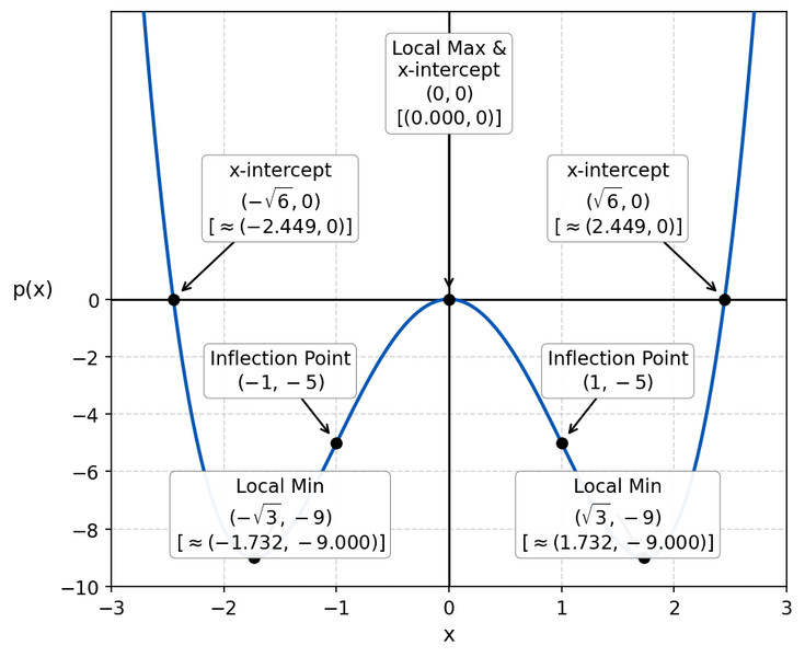
Graph of $p(x)=x^4-6x^2$

Concavity and Points of Inflection

Concavity tells you how the rates of change are changing.

• Concave up means rates of change are increasing. The graph bends upward.
• Concave down means rates of change are decreasing. The graph bends downward.

That gives four possible combinations:

• increasing and concave up
• increasing and concave down
• decreasing and concave up
• decreasing and concave down

A point of inflection is where concavity changes. If it happens at $x=c$, the point is $(c,p(c))$.

A flat point is not automatically an inflection point. The key non-example is $x^4$ at the origin. It’s flat there, but concave up on both sides.

For $p(x)=x^4-6x^2$, the inflection points are $(-1,-5)$ and $(1,-5)$. They are not extrema.

How to Read These Features from Equations, Graphs, and Tables

From an equation, you can identify degree, leading term, and leading coefficient. Rewriting may help. Even degree plus leading coefficient tells you the guaranteed global max or min. Exact extrema or inflection points often need technology.

From a graph:

• left to right rising or falling shows increasing/decreasing
• turning points show local extrema
• changes in bending show concavity and inflection points

From a table:

1. Compute consecutive average rates of change.
2. Look for sign changes in nearby rates for extrema.
3. Look for rates increasing or decreasing for concavity.
4. Look for a reversal in the rate trend for an inflection point.

Common mistakes:

• using output differences when $x$-intervals are unequal
• mixing up local and global
• assuming a zero must be an extremum
• calling any flat point an inflection point