Topic 2.5 Notes – Exponential Function Context and Data Modeling

What an Exponential Model Means

An exponential model describes constant ratio over equal input intervals.

$$f(x)=ab^x$$

• $a$ is the initial value because $f(0)=a$
• $b$ is the factor for each 1-unit increase in input
• growth happens when $b>1$
• decay happens when $0<b<1$

What makes exponential different from linear:

• Linear has a constant difference
• Exponential has a constant ratio

If the input changes by $h$ units, the factor is $b^h$, not just $b$. That’s why equivalent forms matter. A model can show daily growth or weekly growth and still represent the same situation.

Percent change comes from the base:

• growth factor $b=1+r$
• decay factor $b=1-r$
• percent change $=100(b-1)\%$

Common trap: if $b=1.08$, that means 8\% growth, not 108\%.

The natural-base form is also exponential:

$$f(t)=Ae^{kt}$$

• one-unit factor is $e^k$
• growth if $k>0$
• decay if $k<0$

Common trap: $k$ is not the percent change.

Building the Model

There are several ways to create the model, depending on what information you’re given.

From an initial value and factor

If you know the starting amount and the per-unit factor, use

$$f(x)=ab^x$$

If your known point is $(x_i,y_i)$, anchored form is cleaner:

$$f(x)=y_i b^{x-x_i}$$

If the factor applies every $h$ units, use

$$f(x)=y_iR^{(x-x_i)/h}$$

So if something triples every 4 hours and is 900 at $t=0$,

$$C(t)=900\cdot 3^{t/4}$$

From two input-output pairs

If you know $(x_1,y_1)$ and $(x_2,y_2)$, set up

$$y_1=ab^{x_1}, \qquad y_2=ab^{x_2}$$

Divide to eliminate $a$:

$$b=\left(\frac{y_2}{y_1}\right)^{1/(x_2-x_1)}$$

Then find $a$, or write the anchored model directly.

Example with $(3,200)$ and $(7,320)$:

$$b=\left(\frac{320}{200}\right)^{1/4}=(1.6)^{1/4}\approx 1.1247$$

Anchored model:

$$P(t)=200(1.6)^{(t-3)/4}$$

Keep full calculator precision until the end. Early rounding causes wrong later answers.

From a baseline or shifted exponential

Sometimes the quantity approaches a baseline instead of 0:

$$f(x)=L+Ab^{x-h}$$

• $L$ is the baseline or horizontal asymptote
• the exponential part is $f(x)-L$

That means the constant ratio may appear only after adjusting the outputs.

Illustrative examples:

• temperature approaching room temperature
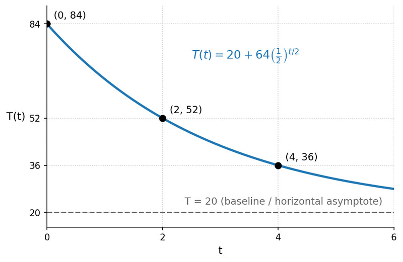
• values 84, 52, 36 with baseline 20

Here, subtract 20:

• $84-20=64$
• $52-20=32$
• $36-20=16$

Now the ratio is constant, so

$$T(t)=20+64\left(\frac12\right)^{t/2}$$

This graph shows the shifted exponential dropping toward the baseline $T=20$.

From technology

For approximately exponential data, use exponential regression. Regression gives a best-fit model, so the curve does not have to pass through every point.

Recognizing Exponential Structure in Data

In a table with equal input spacing:

• constant difference suggests linear
• constant ratio suggests exponential

Ratios only make sense over equal input intervals. That mistake shows up a lot.

Also watch for hidden exponential behavior:

• above-baseline decay means values shrink toward $L$
• below-baseline growth means values rise toward $L$

Common mistakes:

• calling something exponential just because it grows fast
• checking unequal intervals
• forgetting to test $y-L$ instead of raw $y$

Using the Model in Context

To predict an output, substitute the input, then interpret with units. Counts usually round to whole numbers. Measurements depend on context.

To find an input from a target output, solve $ab^x=c$ or $L+Ab^{x-h}=c$ with graphing or numerical technology in this topic. Logarithms come later.

Context matters:

• the mathematical domain may be all real numbers
• the contextual domain may be only $t\ge 0$, or only whole-number times
• interpolation is inside the data range
• extrapolation is outside it and is less reliable

A model prediction is not a guaranteed future value.