Topic 1.7 Notes – Summary Statistics for One Quantitative Variable

What Summary Statistics for One Quantitative Variable Are

A quantitative distribution is a set of numerical data values. Summary statistics give numerical descriptions of three things:

• Center where the data tends to be
• Position where values fall in the ordered list
• Spread how much the data varies

If the data comes from a sample, the numbers are statistics. If they describe an entire population, they are parameters. Right now, you usually work with sample statistics.

No one number tells the whole story. That is why AP Stats usually wants a pair:

• Mean + standard deviation for roughly symmetric data with no strong outliers
• Median + IQR for skewed data or data with outliers

Also know which summaries are resistant to extreme values:

• Resistant: median, quartiles, IQR
• Nonresistant: mean, range, standard deviation

Measures of Center, Position, and Spread

Center

Use this same ordered data set throughout the section so the summary measures connect to one picture.

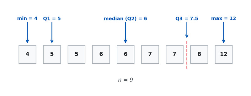
Five-number summary for an ordered data set

The mean uses every value. For a sample,

$$\bar{x}=\frac{\sum x_i}{n}$$

Example with $4,5,5,6,6,7,7,8,12$:

$$\bar{x}=\frac{60}{9}=6.67$$

The mean is the distribution’s balance point. A high outlier can pull it up, so it is nonresistant.

The median is the middle of the ordered data.

• Odd $n$ → the middle value
• Even $n$ → average the two middle values

For the same data, the median is $6$. If the $12$ changed to $30$, the median would still be $6$, which shows why median is resistant.

Position

• Minimum = smallest value
• Maximum = largest value

Quartiles split ordered data into four parts.

• $Q_1$ = median of lower half
• $Q_2$ = median
• $Q_3$ = median of upper half

For AP hand work, when $n$ is odd, you usually exclude the overall median from both halves.

In the ordered list shown above, for $4,5,5,6,6,7,7,8,12$:

• lower half $4,5,5,6$ so $Q_1=5$
• upper half $7,7,8,12$ so $Q_3=7.5$

Percentiles give relative position. The $p$th percentile is the value with $p\%$ of data at or below it.
So $Q_1$, median, $Q_3$ are the 25th, 50th, and 75th percentiles.

Spread

The range is

$$\text{range}=\text{max}-\text{min}$$

Here, $12-4=8$. Range is nonresistant because it only uses endpoints.

The IQR is

$$\text{IQR}=Q_3-Q_1$$

Here, $7.5-5=2.5$. It shows the spread of the middle 50\% and is resistant.

The standard deviation $s$ is the typical distance from the mean:

$$s=\sqrt{\frac{\sum (x_i-\bar{x})^2}{n-1}}$$

You find deviations from the mean, square them, add them, divide by $n-1$, then square root.
$s^2$ is the variance, and variance has squared units.

How to Calculate and Use Them

For median, quartiles, percentiles, range, and IQR, the data must be ordered first. Students lose easy points here all the time.

Interpret in context:

• Median: about half the waiting times were at or below 6 minutes
• IQR: the middle 50% of waiting times spanned 2.5 minutes
• Standard deviation: waiting times typically differed from the mean by about $s$ minutes

On calculator output for sample data, use $S_x$, not $\sigma_x$.

Outliers and Changing Units

Outliers can be flagged two ways. This boxplot uses the 1.5 IQR rule on the waiting-time data and marks 12 as a potential outlier.

• 1.5 IQR rule

$$Q_1-1.5(\text{IQR}),\quad Q_3+1.5(\text{IQR})$$

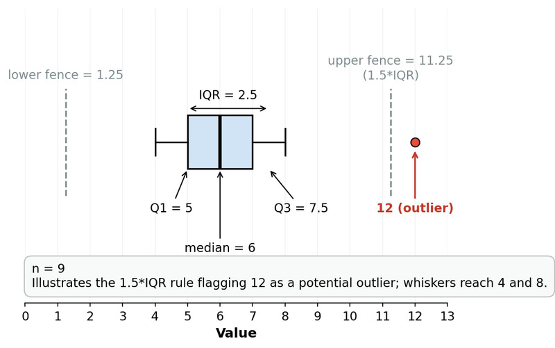
Values beyond the fences are potential outliers. A value exactly on a fence is not.

• Two-standard-deviation rule

$$\bar{x}\pm 2s$$

The two methods can disagree, so say which rule you used. A flagged outlier is not automatically bad data.

If $y=a+bx$:

• center and position stats become $a+b(\text{old stat})$
• range, IQR, and standard deviation multiply by $|b|$
• variance multiplies by $b^2$

Adding a constant changes location but not spread. Multiplying changes both. Linear unit changes do not change which values are flagged as outliers.

Comparing Samples and Common Mistakes

When comparing two independent samples, make direct statements about:

• center
• spread
• shape clues
• outliers

Say something like, “Clinic A has a similar median waiting time but much more variability than Clinic B, since its IQR is larger.”

Summary statistics can hint at skewness or unusual values, but graphs show shape better.