Topic 2.11 Notes – The Normal Distribution

What a Normal Distribution Is

A continuous random variable can take any value in an interval, like height, time, or temperature. Since it can land anywhere, probability comes from intervals, not exact single values.

A normal distribution is a density curve that is:

• continuous
• unimodal with one peak
• bell-shaped
• symmetric

The familiar bell curve also follows the empirical rule shown here.

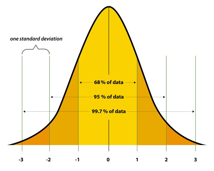
Normal curve and the 68-95-99.7 rule

A few facts all go together here:

• The total area under the curve is 1.
• That means area = probability = proportion = percent.
• For continuous variables, $P(X=a)=0$. A single point has no area.
• So $P(X<a)=P(X\le a)$. Including the endpoint changes nothing.

The curve is determined by two parameters:

• Mean $\mu$ gives the center.
• Standard deviation $\sigma$ gives the spread.

If $X \sim N(\mu,\sigma)$, AP Stats means the second number is the standard deviation, not variance.

Changing $\mu$ shifts the whole curve left or right. Changing $\sigma$ changes width:

• smaller $\sigma$ → narrower and taller
• larger $\sigma$ → wider and shorter

In a normal distribution, mean = median = mode at the center. A normal model is reasonable when data look roughly symmetric, unimodal, and bell-shaped, with no strong skew or extreme outliers.

Z-scores and the Standard Normal

A z-score tells you where a value sits relative to the mean in standard deviation units.

$$z=\frac{x-\mu}{\sigma}$$

• positive $z$ → above the mean
• negative $z$ → below the mean
• larger $|z|$ → farther from the mean, more extreme

The standard normal distribution is $Z \sim N(0,1)$.

Standardizing keeps the normal shape and relative position, but changes the scale. That is why z-scores let you compare values from different distributions.

Example: on a test with $\mu=70$, $\sigma=8$, a score of 86 has

$$z=\frac{86-70}{8}=2$$

So 86 is 2 standard deviations above the mean.

To go backward, use

$$x=\mu+z\sigma$$

If the middle 95% runs from 40 to 64, those are about $\mu-2\sigma$ and $\mu+2\sigma$. The midpoint is $\mu=52$, and $2\sigma=12$, so $\sigma=6$.

The Empirical Rule

For any normal distribution, about:

• 68% of values are within $1\sigma$ of $\mu$
• 95% are within $2\sigma$
• 99.7% are within $3\sigma$

The diagram also breaks that total area into the smaller chunks you will use for quick probability estimates.

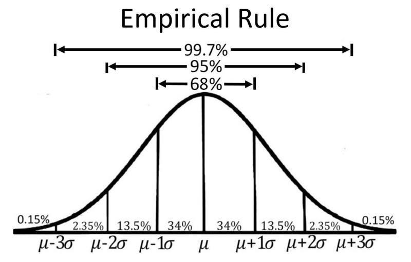
Empirical rule for a normal distribution

Useful split areas:

• $\mu$ to $1\sigma$ on either side → 34%
• $1\sigma$ to $2\sigma$ → 13.5%
• $2\sigma$ to $3\sigma$ → 2.35%
• beyond $3\sigma$ in each tail → 0.15%

This is great for quick estimates and cutoff values like $\mu \pm 2\sigma$. It is only approximate, only for normal distributions, and mostly useful at exactly 1, 2, or 3 standard deviations.

Finding Areas and Finding Cutoffs

When a value is given and you want a probability:

1. Write the probability in context.
2. Decide if it is left-tail, right-tail, or between.
3. If the boundary is exactly 1, 2, or 3 SDs from the mean, use the empirical rule.
4. Otherwise use $z$ or technology.
5. For right-tail area, subtract from 1 if your tool gives left-tail area.

Calculator commands:

• normalcdf(lower, upper, $\mu,\sigma$) for area
• invNorm(left-tail area, $\mu,\sigma$) for cutoffs

When an area is given and you want a value:

• lower $p\%$ means $P(X\le x_a)=p$
• upper $p\%$ means convert to left-tail area $1-p$
• middle $p\%$ means split the leftover area evenly into two tails
• most extreme $p\%$ means split $p\%$ evenly across both tails

Then find $z$, and convert back with $x=\mu+z\sigma$.

Percentiles, Relative Position, and Common Mistakes

The $p$th percentile is the value with about $p\%$ of observations at or below it. So percentile, area, and z-score are all connected:

$x \leftrightarrow z \leftrightarrow$ area/percentile.

To compare positions across distributions, use z-scores or percentiles, not raw values.

Common mistakes show up a lot on tests:

• treating curve height as probability
• using the empirical rule on non-normal data
• forgetting probability is over an interval
• putting an upper-tail percent directly into invNorm
• confusing middle $p\%$ with most extreme $p\%$
• forgetting endpoints do not matter for continuous distributions