Topic 2.12 Notes – Sampling Distributions and the Central Limit Theorem
What a Sampling Distribution Is
A statistic is a number computed from sample data, like or . Since different random samples give different data, the statistic can change too. That change is sampling variability.
A sampling distribution is the distribution of a statistic for all possible samples of one fixed size from one population using one sampling method.
That definition has a lot packed into it. Four things must stay fixed:
- the population
- the sample size
- the statistic
- the sampling method
What changes is the sample itself, so the statistic changes.
Three distributions to keep straight
| Distribution | What it contains |
|---|---|
| Population distribution | values of the variable for all individuals in the population |
| Sample distribution | values from one actual sample |
| Sampling distribution | values of the statistic across many possible samples |
The variable in a sampling distribution is the statistic itself, not the original observations.
Here is a quick example that puts all three ideas side by side.
- Population values might be
- One sample might be
- The sampling distribution of would contain possible sample means like
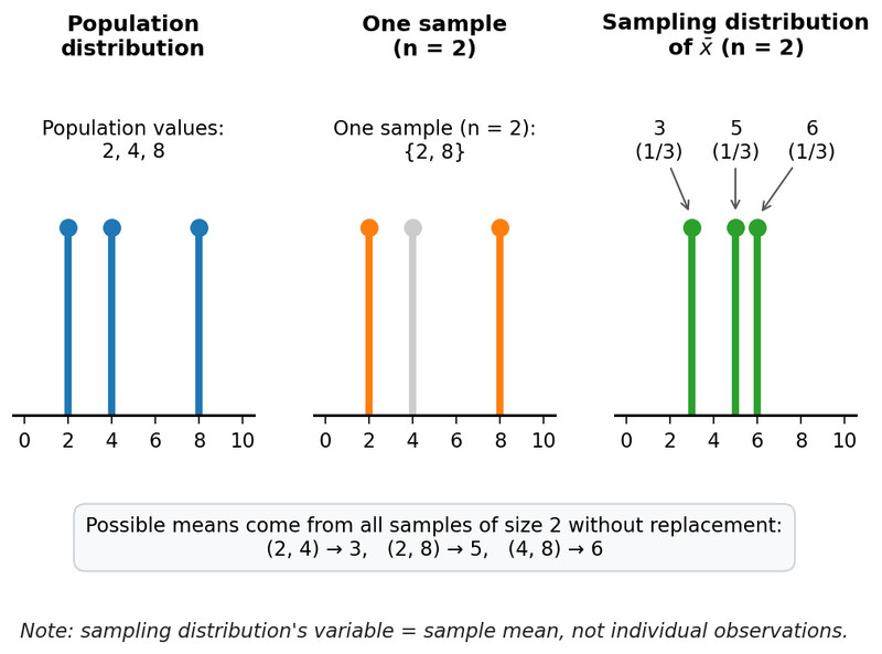
In that last panel, the possible values are sample means from all samples of size 2, not individual data values.
You describe a sampling distribution the same way as any distribution: shape, center, spread, and unusual features. If you change the population, statistic, sample size, or sampling method, you change the sampling distribution.
Simulating a Sampling Distribution
Usually, listing all possible samples is impossible. So we simulate.
How the simulation works
- Specify the population or probability model and any known parameter values.
- Choose a fixed sample size .
- Generate one random sample using the correct process.
- Calculate the statistic.
- Record it.
- Repeat many times.
- Graph the recorded statistics and describe the distribution.
Each dot or bar on the graph represents one statistic from one simulated sample.
What must stay the same every time:
- same population model
- same sample size
- same statistic
- same sampling method, including with or without replacement
A common trap is mixing up sample size and number of repetitions.
- Sample size changes the sampling distribution itself.
- Repetitions only make your simulated graph smoother and more stable.
So if you simulate 5000 samples of size 10, you still have the sampling distribution for , not for a larger sample.
When you describe a simulated sampling distribution, say:
- what statistic it shows
- what sample size was used
- what population/chance model was used
- the shape, center, and spread in context
Randomization Distributions
A randomization distribution comes from repeatedly reassigning observed response values to treatment groups.
This is a different idea from sampling distributions. You are not drawing new samples from a population.
What changes here
- In a simulated sampling distribution, you generate new random samples from a population model.
- In a randomization distribution, you keep the same observed responses and reshuffle the group labels.
How it is built
- Keep the observed response values fixed.
- Randomly reassign them to treatment groups, usually with the same group sizes.
- Recalculate the statistic.
- Record it.
- Repeat and graph the results.
This picture shows one shuffle. The same response values are kept, but they get reassigned to new groups and produce a new difference in means.
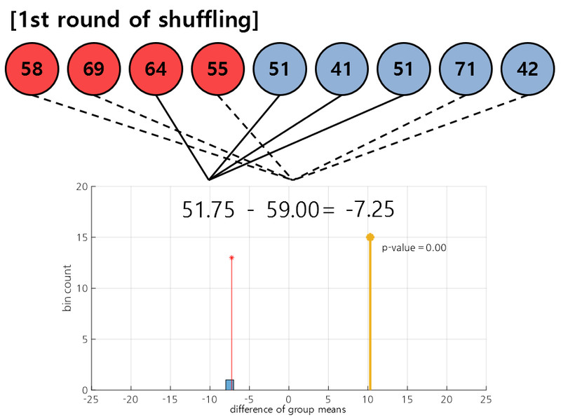
One round of shuffling in a randomization test
The graph below the shuffle shows possible statistic values caused by random assignment alone.
Common AP confusion:
- calling the reassignment process “sampling”
- thinking each point is a new set of responses instead of a new grouping of the same responses
The Central Limit Theorem
The Central Limit Theorem says the sampling distribution of a sample mean can be approximated by a normal distribution, and the approximation improves as gets larger.
This topic is about sample means, not every statistic.
- If the population is normal, the sampling distribution of is normal for any sample size.
- If the population is not normal, larger makes the sampling distribution of more bell-shaped and symmetric.
- Larger also makes sample means less spread out.
The picture below is the classic CLT pattern. It starts with a right-skewed population, then shows how the sampling distribution of changes as increases.
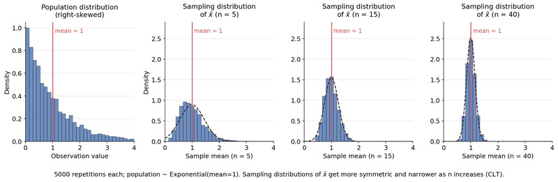
Central Limit Theorem for sample means
Notice that the center stays near the population mean, but the sampling distributions become more symmetric and tighter as the sample size grows.
There is no universal cutoff. is only a rough guideline.
- symmetric population with no outliers → moderate may be enough
- strongly skewed population → need larger
- extreme outliers or heavy tails → may need much larger
Randomness and independence still matter. A huge sample does not fix biased data collection.
What the CLT Does Not Mean
This is where students lose easy points.
- The population does not become normal.
- One large sample of raw data does not have to look normal.
- The CLT does not apply to every statistic.
- Larger samples reduce sampling variability, but they do not erase it.
- More simulation repetitions do not make larger.
Also keep CLT separate from the law of large numbers:
- Law of large numbers means a statistic tends to settle near the true value.
- CLT means the distribution of sample means across repeated samples tends toward normality.
Key Takeaways
Sampling Distribution
Distribution of a statistic’s values for all possible samples of a fixed size from a given population using the same random sampling process
Sampling Variability
Sample-to-sample variation in a statistic when different random samples are selected
Population Distribution vs Sample Distribution vs Sampling Distribution
Population distribution: values of a variable for the whole population; sample distribution: values in one sample; sampling distribution: values of a statistic across all possible same-size samples
Simulated Sampling Distribution
Approximation of a sampling distribution made by repeatedly taking random samples from a population or model, calculating the statistic, and recording it
Steps To Simulate a Sampling Distribution
Specify population/model and parameter values, choose fixed n, generate a random sample, calculate the statistic, record it, repeat many times, and graph the recorded statistics
Sample Size vs Number Of Repetitions
Sample size is the number of observations in each sample; repetitions are the number of simulated statistics used to approximate the distribution
Randomization Distribution
Distribution of a statistic generated by repeatedly randomly reallocating or reassigning observed response values to treatment groups and recalculating the statistic
Sampling Distribution vs Randomization Distribution
Sampling distribution comes from repeatedly drawing new random samples from a population or model; randomization distribution comes from repeatedly reassigning existing response values to treatment labels
Central Limit Theorem
For the mean x̄ of a random sample, the sampling distribution can be approximated by a normal distribution; the larger the sample size, the better the approximation
What The Central Limit Theorem Applies To
The theorem applies to the sampling distribution of the sample mean x̄, not to the population distribution or the data in one sample
Effect Of Larger Sample Size On The Sampling Distribution Of x̄
As n increases, the sampling distribution of x̄ becomes less spread out; if the population is not normal, it also becomes more nearly symmetric and bell-shaped
Law Of Large Numbers vs Central Limit Theorem
Law of large numbers: a long-run average gets closer to its expected value; central limit theorem: the sampling distribution of sample means becomes approximately normal as n increases
Random Sample
Sample selected by a random process so the observations can be treated as representative draws from the population model
Notes
Sampling Distribution
Distribution of a statistic’s values for all possible samples of a fixed size from a given population using the same random sampling process
Sampling Variability
Sample-to-sample variation in a statistic when different random samples are selected
Population Distribution vs Sample Distribution vs Sampling Distribution
Population distribution: values of a variable for the whole population; sample distribution: values in one sample; sampling distribution: values of a statistic across all possible same-size samples
Simulated Sampling Distribution
Approximation of a sampling distribution made by repeatedly taking random samples from a population or model, calculating the statistic, and recording it
Steps To Simulate a Sampling Distribution
Specify population/model and parameter values, choose fixed n, generate a random sample, calculate the statistic, record it, repeat many times, and graph the recorded statistics
Sample Size vs Number Of Repetitions
Sample size is the number of observations in each sample; repetitions are the number of simulated statistics used to approximate the distribution
Randomization Distribution
Distribution of a statistic generated by repeatedly randomly reallocating or reassigning observed response values to treatment groups and recalculating the statistic
Sampling Distribution vs Randomization Distribution
Sampling distribution comes from repeatedly drawing new random samples from a population or model; randomization distribution comes from repeatedly reassigning existing response values to treatment labels
Central Limit Theorem
For the mean x̄ of a random sample, the sampling distribution can be approximated by a normal distribution; the larger the sample size, the better the approximation
What The Central Limit Theorem Applies To
The theorem applies to the sampling distribution of the sample mean x̄, not to the population distribution or the data in one sample
Effect Of Larger Sample Size On The Sampling Distribution Of x̄
As n increases, the sampling distribution of x̄ becomes less spread out; if the population is not normal, it also becomes more nearly symmetric and bell-shaped
Law Of Large Numbers vs Central Limit Theorem
Law of large numbers: a long-run average gets closer to its expected value; central limit theorem: the sampling distribution of sample means becomes approximately normal as n increases
Random Sample
Sample selected by a random process so the observations can be treated as representative draws from the population model
