Topic 2.9 Notes – Parameters of Random Variables

What the Parameters of a Discrete Random Variable Are

A discrete random variable $X$ has countable possible values, and each value has a probability. Those probabilities must all be between 0 and 1 and add up to 1.

A parameter is a fixed numerical characteristic of a population or probability distribution. For a discrete random variable $X$, the main parameters here are:

• Mean $E(X)=\mu_X$
• Variance $V(X)=\sigma_X^2$
• Standard deviation $SD(X)=\sigma_X$

The subscript matters. $\mu_X$ means the mean of the distribution of that random variable $X$.

One easy confusion to avoid:

• Outcome of $X$ changes from trial to trial.
• Parameters of the distribution stay fixed.
• Statistics like $\bar{x}$ and $s$ come from sample data, so they can change from sample to sample.

Mean, Variance, and Standard Deviation

Mean or expected value

The expected value is the probability-weighted average of the possible values.

$$\mu_X=E(X)=\sum x_iP(X=x_i)$$

That means each outcome gets multiplied by how likely it is, then you add.

• It gives the long-run average over many repetitions.
• It has the same units as $X$.
• It is not the guaranteed result of one trial.
• It might not be the most likely value.
• It does not even have to be a possible outcome.

You can also think of the mean as the distribution’s balance point.

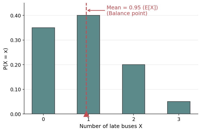
Mean as a distribution’s balance point

Variance

Variance measures how spread out the distribution is around the mean.

$$\sigma_X^2=V(X)=\sum (x_i-\mu_X)^2P(X=x_i)$$

The squared deviations do two jobs:

• they keep positive and negative deviations from canceling
• they give more weight to values far from the mean

Variance has squared units, so it is usually less meaningful in context.

Standard deviation

Standard deviation is the square root of variance.

$$\sigma_X=SD(X)=\sqrt{\sum (x_i-\mu_X)^2P(X=x_i)}$$

This is the typical distance of values of $X$ from the mean in the long run. It has the same units as $X$.

• Larger $\sigma_X$ means more spread
• $\sigma_X=0$ means $X$ always takes one value

Equivalent variance shortcut

Sometimes arithmetic is faster with

$$V(X)=E(X^2)-[E(X)]^2$$

where

$$E(X^2)=\sum x_i^2P(X=x_i)$$

Use this when the numbers are annoying, but the original variance formula shows the meaning better.

How to Calculate Them from a Probability Distribution

Suppose $X$ is the number of late buses in a morning, with:

• 0 with probability 0.35
• 1 with probability 0.40
• 2 with probability 0.20
• 3 with probability 0.05

First check it’s valid. All probabilities are between 0 and 1, and $0.35+0.40+0.20+0.05=1$.

A table like this helps organize the mean and variance calculations.

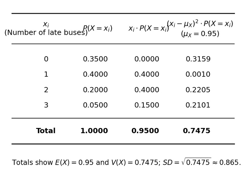
Probability distribution table with mean, variance, and standard deviation calculations

Then calculate:

1. Mean

   $$\mu_X=0(0.35)+1(0.40)+2(0.20)+3(0.05)=0.95$$

2. Variance using the exact mean

   $$\sigma_X^2=(0-0.95)^2(0.35)+(1-0.95)^2(0.40)+(2-0.95)^2(0.20)+(3-0.95)^2(0.05)=0.7475$$

3. Standard deviation

   $$\sigma_X=\sqrt{0.7475}\approx0.865$$

On technology, put values in one list and probabilities in a weight/frequency list. Use weighted 1-variable stats and choose population standard deviation $\sigma_x$, not sample $s_x$.

How to Interpret the Mean and Standard Deviation

Your answer has to be in context.

• Mean
  Over many mornings, the long-run average number of late buses will be about $0.95$ late buses per morning.

• Standard deviation
  Over many mornings, the number of late buses will typically differ from its mean of $0.95$ by about $0.865$ bus.

Together, these tell you:

• mean gives center
• standard deviation gives spread around that center

They do not tell you the full shape by themselves.

Common Mistakes and Exam Traps

• Saying the expected value is what will happen on one trial
• Treating the expected value as the most likely outcome
• Forgetting the expected value can be non-integer even if $X$ counts things
• Giving variance when the question asked for standard deviation
• Rounding $\mu_X$ too early before finding $\sigma_X$
• Leaving out context, units, or long-run language in interpretation
• Mixing up distribution parameters $\mu_X,\sigma_X$ with sample statistics $\bar{x},s$