Topic 2.8 Notes – Introduction to Random Variables and Probability Distributions

What a Random Variable and Its Distribution Are

A random variable is the numerical result of a random process. You’ll usually see the variable written with a capital letter, like $X$, and one possible value written in lowercase, like $x$. So $P(X=x)$ means “the probability that random variable $X$ takes value $x$.”

What matters is that you define $X$ in context. Example:

• Roll two four-sided dice.
• $X=$ the sum of the rolls
• $Y=$ the larger roll
• $Z=$ the absolute difference of the rolls

Same process, different variables, different distributions.

A common trap is mixing up an outcome with a random-variable value. If $Z$ is the absolute difference, then $(1,4)$ and $(4,1)$ are different outcomes, but both give $Z=3$. That means their probabilities get combined.

This topic is about discrete random variables. That means the possible values are separate and countable.

• They might be whole numbers, like 0, 1, 2, 3.
• They do not have to be whole numbers. Values like 0, 2.5, and 10 are still discrete if those are the only possible amounts.

A probability distribution lists every possible value and its probability.

It is valid only if:

• each probability is between 0 and 1
• all probabilities add to 1

How to Construct a Discrete Probability Distribution

This is where students often lose points by stopping at sample-space outcomes instead of regrouping by the random variable.

1. Define the variable clearly in context.
2. List all possible values of the variable.
3. Find which outcomes produce each value.
4. Use probability rules to get those probabilities.
5. Add probabilities of different outcomes that lead to the same value.
6. Check that the probabilities sum to 1.

Example with two fair four-sided dice. Let $X=$ absolute difference.

Possible values are $0,1,2,3$.

• $X=0$ from $(1,1),(2,2),(3,3),(4,4)$ so $P(X=0)=4/16$
• $X=3$ from $(1,4),(4,1)$ so $P(X=3)=2/16$

And so on for 1 and 2.

If one probability is missing, use

$$\text{sum of all probabilities} = 1$$

So if probabilities are $0.18, 0.27, k, 0.31$, then

$$0.18+0.27+k+0.31=1$$

so $k=0.24$.

Ways to Represent the Distribution

The same distribution can be shown three ways.

Probability tables

A table pairs each possible value with its probability. It must include every possible value.

Graphs of discrete distributions

The horizontal axis shows variable values. The vertical axis shows probability.

For the absolute difference of two four-sided dice, the graph looks like this.

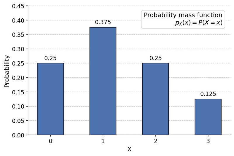
Probability distribution for $X=$ absolute difference of two four-sided dice

The bars are separated because the values are discrete. If the axis shows counts instead, that is not a probability distribution unless it is clearly simulated relative frequency.

Probability functions

You may also see

$$p_X(x)=P(X=x)$$

That notation appears in the graph too. Sometimes it’s written piecewise, and impossible values can be given probability 0.

Building a Distribution from Simulation

Simulation is useful when exact calculation is hard.

• simulate one full trial
• record the random-variable value
• repeat many times
• count each value
• divide by total trials

Those results are estimates, not exact probabilities. More repetitions usually make them closer to the true distribution.

Using the Distribution and the Cumulative Distribution

Once you have the distribution, event probabilities come from adding the probabilities of values that fit the condition.

• exactly $a$ means $X=a$
• at most $a$ means $X\le a$
• at least $a$ means $X\ge a$
• fewer than $a$ means $X<a$
• more than $a$ means $X>a$

For discrete variables, endpoints matter.

The cumulative distribution is

$$F(x)=P(X\le x)$$

You build it by adding from the bottom up. It never goes down and ends at 1. This step graph shows that each jump happens at a possible value of $X$, and each flat stretch means the cumulative probability stays the same between values.

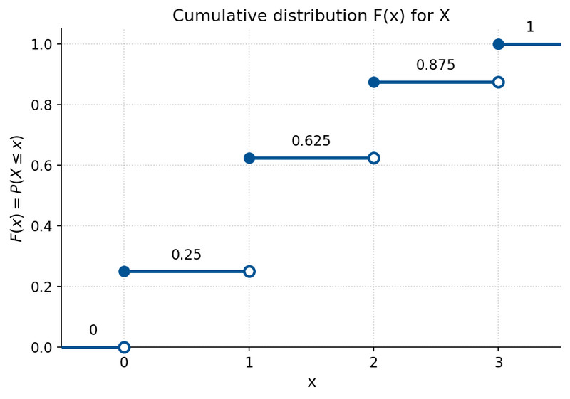
Cumulative distribution function for a discrete random variable

This is the difference students confuse all the time:

• $P(X=x)$ means one exact value
• $F(x)=P(X\le x)$ means that value and everything below it

Useful shortcuts:

$$P(X>b)=1-F(b)$$

$$P(a<X\le b)=F(b)-F(a)$$