Topic 4.2 Notes – Constructing a Confidence Interval for a Population Mean or Population Mean Difference

What a One-Sample t-Interval Is

A one-sample t-interval estimates an unknown population mean $\mu$ when $\sigma$ is unknown, so you use the sample standard deviation $s$ instead.

The full form is

$$\bar{x} \pm t^*\left(\frac{s}{\sqrt{n}}\right)$$

That breaks into familiar pieces:

• Point estimate is $\bar{x}$, the sample mean.
• Standard error is

$$\text{SE}=\frac{s}{\sqrt{n}}$$

• Margin of error is

$$\text{ME}=t^*\times \text{SE}$$

So the interval is just estimate ± wiggle room.

For matched pairs, you do not run a two-sample method here. You first compute a difference for each pair, then treat those differences as one sample. The parameter becomes $\mu_d$, the population mean of the paired differences, and you must say the subtraction order in words.

Why t-Distributions Are Used

If $\sigma$ were known, mean inference would use a normal $z$-procedure. In real life, $\sigma$ is usually unknown, so using $s$ adds extra uncertainty. That is why you use a t-distribution.

A t-distribution is:

• symmetric
• bell-shaped
• centered at 0
• standardized

Compared with the standard normal curve, t-curves have:

• lower peaks
• heavier tails

This graph shows that shape difference for a t-curve with very small degrees of freedom.

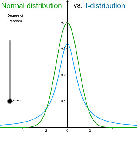
Those heavier tails account for the extra uncertainty from estimating $\sigma$ with $s$.

There is a whole family of t-curves, identified by degrees of freedom. For a one-sample t-procedure,

$$\text{df}=n-1$$

As df gets larger, the t-curve gets closer to the standard normal curve. Because of the heavier tails, the critical value $t^*$ is usually larger than the matching $z^*$.

Choosing the Right Mean Interval

The first question is about the design.

One sample

This means one quantitative measurement from each person or object.

• Procedure used: one-sample t-interval for a population mean
• Parameter: $\mu$, the population mean of the quantitative variable in context

Example. $\mu$ could be “the mean battery life of all batteries of this model.”

Matched pairs

This means the same individuals measured twice or naturally paired individuals.

• Compute differences first
• Use a one-sample t-interval for a population mean difference
• Parameter: $\mu_d$

Be careful here:

• If you define difference as before minus after, keep that order the whole time.
• Reversing the order changes the sign of $\bar{d}$ and both interval endpoints.
• $n$ is the number of pairs, not the total number of raw values.

Two independent groups belong to a two-sample t-interval, which is outside this topic.

Conditions for Using a One-Sample t-Interval

You need all the usual checks, and each one has a different job.

• Randomization
  • Data come from a random sample or randomized experiment.
  • On an FRQ, say how you know. Example: “A simple random sample of 25 students was selected.”
• 10% condition
  • When sampling without replacement from a finite population, check

$$n \le 0.10N$$

• This supports independence, not normality.
• Usually unnecessary in randomized experiments.

• Sample data condition
  • Population is approximately normal, or $n \ge 30$, or if $n<30$, the sample shows no strong skewness or outliers.
  • For matched pairs, check the differences, not the two original lists.

This is where the shape of the data matters. For small samples, a roughly symmetric distribution is usually fine. Strong skewness or clear outliers are a warning sign.

A common trap is mixing up $n \ge 30$ with the 10% condition. They are different checks for different reasons.

Building the Interval and Avoiding Common Mistakes

Here is the full flow you’ll actually use:

1. Define the parameter in context.
2. Decide whether this is one sample or matched pairs.
3. Verify conditions.
4. Compute $\text{df}=n-1$.
5. Find $t^*$ from the confidence level and df.
6. Compute $\text{SE}=\frac{s}{\sqrt{n}}$ or $\frac{s_d}{\sqrt{n}}$.
7. Compute $\text{ME}=t^*\times \text{SE}$.
8. Write the interval as $\bar{x}\pm \text{ME}$ or $\bar{d}\pm \text{ME}$, with units.

Quick example. If $\bar{x}=52.4$, $s=6.8$, $n=16$, and $t^*=2.131$, then

$$\text{SE}=\frac{6.8}{\sqrt{16}}=1.7$$

$$\text{ME}=2.131(1.7)=3.6227$$

So the interval is $52.4 \pm 3.6227$, or about $(48.8, 56.0)$.

Common mistakes show up a lot:

• using $z^*$ instead of $t^*$
• using $s$ instead of $\frac{s}{\sqrt{n}}$
• checking paired variables instead of the differences
• using total observations instead of number of pairs
• forgetting to define subtraction order for $\mu_d$
• rounding too early and changing the endpoints