Topic 4.4 Notes – Setting Up a Test for a Population Mean or Population Mean Difference

What a One-Sample t-Test Tests

A one-sample t-test is used when the variable is quantitative and you want to test a claim about a single population mean, written as $\mu$.

Why t and not z? Because $\sigma$, the population standard deviation, is unknown. You estimate it with the sample standard deviation $s$, and that extra uncertainty is handled by the t-distribution.

For these tests, the degrees of freedom are

$$\text{df} = n - 1$$

Two versions show up in this topic:

• One sample of quantitative data
  • You test a single population mean $\mu$.
• Matched pairs
  • You turn each pair into one difference.
  • Then you test the population mean of those differences, $\mu_d$.

This is the basic decision tree for this part of inference. For this section, focus on the left branch for one sample vs. a known value and the right branch for paired or matched observations.

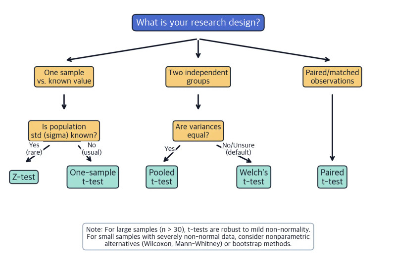
t-test decision tree

This is not for:

• categorical data or proportions
• two independent samples
• comparing two separate groups with no pairing

Choosing the Right Setup

The first question is what kind of data structure you have.

One quantitative sample

Use this when there is one random sample and the claim is about that population’s mean.

Your parameter should sound like this:

• $\mu =$ the true mean of the quantitative variable for the population in context

Example:

• $\mu =$ the true mean fill weight of all cereal boxes produced today

Matched pairs

Use this when observations are dependent, like:

• before and after on the same person
• the same subject under two treatments
• matched individuals
• natural pairs such as twins

You define a difference for each pair, such as

$$d = B - A$$

Then you analyze the single sample of differences with a one-sample t-test.

Your parameter becomes:

• $\mu_d =$ the true mean of the pairwise differences in context

Order of subtraction

This part is easy to mess up. If you define $d = B - A$, then positive differences mean $B$ tends to be larger than $A$. If you switch to $A - B$, every sign flips, so the direction of the alternative flips too.

The claim has to match your defined difference, not just the wording in the prompt.

Writing the Parameter and Hypotheses

Your parameter definition needs all three pieces:

• the population
• the quantitative response variable
• the mean parameter

Example:

• $\mu =$ the true mean resting heart rate of all students at this school

One-sample hypotheses

$$H_0:\mu=\mu_0$$

$$H_a:\mu<\mu_0,\quad \mu>\mu_0,\quad \text{or}\quad \mu\ne\mu_0$$

Matched-pairs hypotheses

$$H_0:\mu_d=0$$

$$H_a:\mu_d<0,\quad \mu_d>0,\quad \mu_d\ne0$$

Tail choice comes from the claim:

• “lower,” “decreased,” “less than” → left-tailed
• “higher,” “increased,” “greater than” → right-tailed
• “different,” “changed” → two-tailed

Common mistakes:

• using $\bar{x}$ or $\bar{d}$ in hypotheses instead of $\mu$ or $\mu_d$
• putting equality in $H_a$
• choosing the tail based on sample results

Conditions for a One-Sample t-Test

You need three conditions.

Randomization

The data should come from a random sample or a randomized experiment. In matched pairs, dependence within a pair is fine.

10% condition

When sampling without replacement,

$$\frac{n}{N} \le 0.10 \quad \text{or} \quad N \ge 10n$$

For matched pairs, $n$ is the number of pairs.

Sample data condition

You can use the test if:

• the population is approximately normal, or
• $n \ge 30$, or
• if $n < 30$, the sample data show no strong skewness or outliers

For matched pairs, check the differences, not the two original samples. That means you should make your normality and outlier decision from the distribution of the pairwise differences.

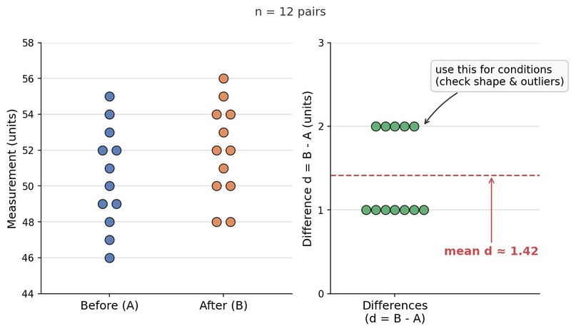
Matched-pairs conditions: check the differences

The Setup Sequence on the Exam

A clean AP Stats setup usually goes in this order:

1. Define the parameter in context.
2. If paired, define $d$ and say the subtraction order.
3. Write $H_0$ and $H_a$ using $\mu$ or $\mu_d$.
4. Name the procedure.
   • one-sample t-test for a population mean
   • one-sample t-test for a population mean difference
5. Check randomization, 10%, and sample data conditions.
6. If $\alpha$ is given, mention it, but it does not decide the hypotheses or conditions.

Biggest setup errors:

• treating paired data as independent samples
• forgetting to define the difference
• checking shape on the raw data instead of on the differences
• trying to compute the test statistic or p-value during setup