Topic 4.5 Notes – Carrying Out a Test for a Population Mean or Population Mean Difference

The One-Sample t-Test for a Mean or Mean Difference

A one-sample t-test is used when you want to test a population mean $\mu$ and the population standard deviation $\sigma$ is unknown. That’s why this is a t procedure instead of a z procedure. You use the sample standard deviation $s$ to estimate $\sigma$.

For matched pairs, you do one more step first. Turn each pair into a single difference, then test the population mean of those differences, $\mu_d$. After that, it is still a one-sample t-test.

$$t=\frac{\bar{x}-\mu_0}{s/\sqrt{n}}, \qquad \text{df}=n-1$$

For paired data,

$$t=\frac{\bar{x}_d-\mu_{d,0}}{s_d/\sqrt{n}}, \qquad \text{df}=n-1$$

Usually for paired data, $\mu_{d,0}=0$.

What the t-statistic means:

• It tells you how many estimated standard errors your sample mean is from the null value.
• Positive $t$ means the sample mean is above the null value.
• Negative $t$ means the sample mean is below the null value.
• The sign always matches $\bar{x}-\mu_0$, or $\bar{x}_d-\mu_{d,0}$ for pairs.

When you find a P-value, you use the t-distribution and look at the tail area beyond your test statistic. This graph shows a two-sided test, with equal shaded areas in both tails for $t$-values equally far from 0.

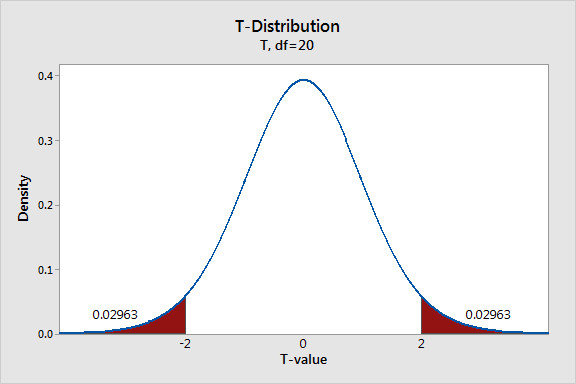
Two-tailed P-value on a t-distribution

Conditions and Setup You Still Need to Carry Through

Even though this topic is about calculations and conclusions, a complete test still includes the earlier setup:

• parameter
• hypotheses
• procedure name
• conditions

The conditions are the same ones you’ve been checking:

• Random
  Data came from a random sample or randomized experiment.
• Independence
  If sampling without replacement, use the 10% condition. $n \le 0.10N$
• Sample data condition for t procedures
  • If population is approximately normal, okay.
  • If $n \ge 30$, usually okay unless the distribution is extremely skewed.
  • If $n < 30$, the sample data should have no strong skewness and no outliers.

For matched pairs, check the shape of the differences, not the two original lists.

Good graph language sounds like this:

• “The distribution of sample differences is roughly symmetric with no apparent outliers.”

That is much better than just saying “it looks normal.”

This topic is not the two-sample t-test for two independent means.

Carrying Out the Test

Here’s the flow of the calculation.

1. Compute the estimated standard error.
   $\frac{s}{\sqrt{n}}$ or $\frac{s_d}{\sqrt{n}}$
2. Calculate the test statistic.
   Report $t$ and $df=n-1$.
3. Find the p-value using the alternative hypothesis, not the sample result.

• If $H_a:\mu>\mu_0$, use $P(T \ge t_{obs})$
• If $H_a:\mu<\mu_0$, use $P(T \le t_{obs})$
• If $H_a:\mu\ne\mu_0$, use $P(|T|\ge |t_{obs}|)$

Quick example

Suppose $\bar{x}=18.2$, $s=4.5$, $n=25$, and $H_0:\mu=16$.

$$t=\frac{18.2-16}{4.5/\sqrt{25}}=\frac{2.2}{0.9}\approx 2.44$$

So $df=24$. If $H_a:\mu>16$, the p-value is the right-tail probability for $t=2.44$ with 24 df.

Using a t-table

• Use the row for $df=n-1$.
• Most tables give upper-tail areas.
• For a two-sided test, double the one-tail area.
• If your exact df is missing, use the next smaller df. That gives a conservative p-value.

Using technology

Enter:

• $\mu_0$
• $\bar{x}$
• $s$
• $n$
• correct alternative

Still show the formula setup in your work.

Interpreting the p-Value and Making the Decision

A p-value is the probability, assuming $H_0$ is true, of getting a result as extreme or more extreme than the one observed, in the direction of $H_a$.

A strong AP Stats interpretation includes:

• the null assumption
• “as extreme or more extreme”
• the direction from the alternative
• the parameter and variable in context
• the random process

Example in context:

• “If the true mean fill weight of all cereal boxes from this shift is 500 grams, then the probability of getting a sample mean at least this far from 500 grams, in either direction, from a random sample of 25 boxes is 0.0245.”

Decision rule:

• If p-value $\le \alpha$, reject $H_0$
• If p-value $> \alpha$, fail to reject $H_0$

Statistical significance means evidence against $H_0$. It does not tell you the effect is large or important.

Writing the Conclusion and Avoiding Common Mistakes

Use AP-style wording.

• If you reject
  “Because the p-value is less than or equal to $\alpha$, reject $H_0$. There is convincing evidence that...”
• If you fail to reject
  “Because the p-value is greater than $\alpha$, fail to reject $H_0$. There is not convincing evidence that...”

Your conclusion must name:

• the population
• the response variable
• the parameter
• the direction or difference from $H_a$

For matched pairs, be careful:

• Define the subtraction order.
• Reversing the order flips the signs of $\bar{x}_d$, $t$, and the directional alternative.
• $n$ is the number of pairs, not total measurements.

Common mistakes:

• using the wrong tail(s)
• choosing $H_a$ from the sample direction
• saying “the null is true” or “the null is false”
• concluding “greater than” when $H_a$ was “different from”
• treating paired data like two independent samples