Topic 4.6 Notes – Sampling Distributions for the Difference Between Two Sample Means

What the Sampling Distribution of $\bar{x}_1 - \bar{x}_2$ Is

You have two independent groups or populations, one quantitative variable, and two sample means, $\bar{x}_1$ and $\bar{x}_2$. The statistic is their difference:

$$\bar{x}_1-\bar{x}_2$$

That statistic estimates the population difference:

$$\mu_1-\mu_2$$

The subtraction order matters the whole time. If population 1 is “students using Method A” and population 2 is “students using Method B,” then keep that order for both sample means and population means.

A sampling distribution is the distribution of $\bar{x}_1-\bar{x}_2$ from many repeated independent samples. It is about sample means, not individual data values.

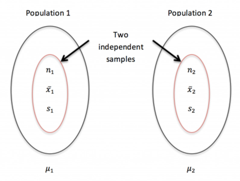
Two independent samples from two populations

The diagram shows the setup. You draw one independent sample from population 1 and another from population 2, then compare their sample means.

The center is

$$\mu_{\bar{x}_1-\bar{x}_2}=\mu_1-\mu_2$$

So $\bar{x}_1-\bar{x}_2$ is an unbiased estimator of $\mu_1-\mu_2$. If $\mu_1=\mu_2$, the sampling distribution is centered at 0, even though actual sample differences will bounce above and below 0.

Spread and Shape of the Sampling Distribution

The standard deviation of the sampling distribution is

$$\sigma_{\bar{x}_1-\bar{x}_2}=\sqrt{\frac{\sigma_1^2}{n_1}+\frac{\sigma_2^2}{n_2}}$$

Here’s the part students mix up a lot. Variances add for independent random variables, even when you subtract the variables. That’s why the formula adds $\frac{\sigma_1^2}{n_1}$ and $\frac{\sigma_2^2}{n_2}$.

• You do not add or subtract standard deviations directly.
• The spread is in the same units as the original variable.
• Bigger $n_1$ or $n_2$ makes the sampling distribution tighter.
• The population with larger $\sigma^2/n$ contributes more to the total spread.

For the shape, $\bar{x}_1-\bar{x}_2$ is:

• Exactly normal if both population distributions are normal
• Approximately normal if both sample sizes are large, meaning $n_1 \ge 30$ and $n_2 \ge 30$

Both samples have to meet the large-sample condition. One large sample does not rescue one small sample.

Full model:

$$\bar{x}_1-\bar{x}_2 \sim N\left(\mu_1-\mu_2,\sqrt{\frac{\sigma_1^2}{n_1}+\frac{\sigma_2^2}{n_2}}\right)$$

Conditions to Check Before Using the Model

You need to justify independence and normal shape.

Independence conditions

• For sampling, you need two independent random samples
• For experiments, you need random assignment to independent groups
• This is not for matched pairs or repeated measures. Those use paired-data methods.

The 10% condition

This only matters for sampling without replacement from populations.

Check each sample separately:

• $n_1 \le 0.10N_1$
• $n_2 \le 0.10N_2$

You compare each sample to its own population, not a combined sample to a combined population. Randomized experiments do not need the 10% condition.

What to say on an exam

Name the randomization source from the prompt, say the two samples or groups are independent, check 10% separately if sampling, and justify normality with either normal populations or both sample sizes at least 30.

Finding and Interpreting Probabilities

Only do probability calculations after the normal model is justified.

Standardize with

$$z=\frac{(\bar{x}_1-\bar{x}_2)-(\mu_1-\mu_2)}{\sqrt{\frac{\sigma_1^2}{n_1}+\frac{\sigma_2^2}{n_2}}}$$

For a cutoff $c$,

$$z=\frac{c-(\mu_1-\mu_2)}{\sqrt{\frac{\sigma_1^2}{n_1}+\frac{\sigma_2^2}{n_2}}}$$

Example. Suppose $\mu_1=78$, $\mu_2=74$, $\sigma_1=12$, $\sigma_2=10$, $n_1=64$, $n_2=100$.

Then

$$\mu_{\bar{x}_1-\bar{x}_2}=78-74=4$$

$$\sigma_{\bar{x}_1-\bar{x}_2}=\sqrt{\frac{12^2}{64}+\frac{10^2}{100}}=\sqrt{2.25+1}=\sqrt{3.25}\approx1.803$$

For $P(\bar{x}_1-\bar{x}_2>7)$,

$$z=\frac{7-4}{1.803}\approx1.66$$

So $P(Z>1.66)\approx0.048$.

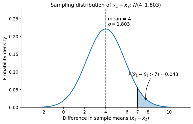
In context, you’d say there is about a 0.048 probability that repeated independent samples of 64 and 100 students would produce a sample mean score difference greater than 7 points.

What Students Mix Up

• Using this for paired data instead of independent groups
• Flipping the subtraction order halfway through
• Describing the distribution as if it were about individual observations
• Forgetting both samples need normal populations or both need $n \ge 30$
• Using the 10% condition for experiments
• Using $s_1$ and $s_2$ here. This topic uses population SDs, $\sigma_1$ and $\sigma_2$
• Treating probability as about $\mu_1-\mu_2$. The parameter is fixed and the statistic varies
• Thinking large samples fix bad sampling or confounding