Topic 2.10 Notes – The Binomial Distribution
What a Binomial Random Variable Is
A binomial random variable is a discrete random variable that counts successes in a fixed number of trials. If , then:
- = number of trials
- = probability of success on each trial
- can be
“Success” just means the outcome you’re counting. It could be a made shot, a defective product, or a missed question.
BINS conditions
For a variable to be binomial, all four must hold:
- Binary: each trial is labeled success or failure
- Independent: one trial doesn’t change another
- Number: the number of trials is fixed ahead of time
- Same probability: stays constant
A couple of easy traps:
- A trial can have several actual outcomes and still be binomial if you group them into success/failure.
- Example: “uses a credit card” vs “does not use a credit card”
- “Number of successes in the next 12 trials” can be binomial.
- “How many trials until the first success” is not binomial because the number of trials is not fixed.
- Without replacement is not truly independent, but it’s close enough if the sample is no more than 10% of the population.
When you justify binomial on a test, say it in context. Example:
- Let be the number of defective bulbs in the next 20 bulbs checked.
- Each bulb is defective or not defective.
- The checks are independent.
- There are 20 bulbs, fixed in advance.
- The probability a bulb is defective is each time.
So .
Finding Binomial Probabilities
The exact probability of getting exactly successes is
Here’s what the pieces mean:
- counts how many ways the successes can be arranged
- accounts for the successes
- accounts for the failures
For example, if , this probability model is centered around 3 successes, and the graph helps you see which counts are most likely.
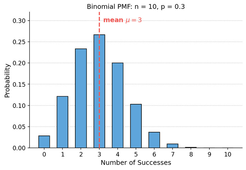
If , then
Calculator shortcuts matter a lot here:
- gives
- gives
Translating words into probability notation
- exactly
- at most
- fewer than
- at least
- more than
- between and , inclusive
Upper-tail probabilities are usually fastest with complements:
Be careful. equals , not .
Mean and Standard Deviation of a Binomial Distribution
For ,
If , then
- mean
- standard deviation
Interpret them in context:
- The mean is the long-run average number of defective bulbs in many groups of 20.
- The standard deviation is the typical distance that count is from 1.6 bulbs.
A common mistake is using as the standard deviation. That’s the variance. Also, the mean can be non-integer even though the count itself must be whole numbers.
For fixed , spread is biggest near and smaller when is near 0 or 1.
Estimating Binomial Probabilities with Simulation
Simulation works when you build the same trial structure as the binomial setting.
- Create a chance model with probability of success.
- Run independent trials.
- Count successes. That count is one simulated value of .
- Repeat many times.
- Use relative frequency to estimate probability.
Here’s what that looks like for and :
- Let digits 1-2 = success, 3-0 = failure.
- Generate 5 random digits for one repetition.
- If the digits are 1, 7, 2, 9, 4, then .
- After many repetitions, estimate by the proportion with exactly 2 successes.
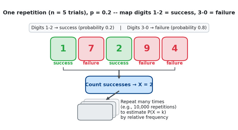
Binomial simulation with random digits
One repetition is the full set of trials, not one trial. That mistake shows up a lot.
Key Takeaways
Binomial Random Variable
A discrete random variable that counts the number of successes in a fixed number n of independent trials with binary outcomes and the same success probability p
X ~ Bin(n, p)
Notation that X has a binomial distribution with n trials and probability of success p on each trial
BINS
Binary outcomes, Independent trials, fixed Number of trials, Same probability of success on each trial
Success
The outcome being counted in a binomial setting; it need not be desirable
Binomial Probability Function
P(X = x) = (n choose x)p^x(1 − p)^(n − x), for x = 0, 1, ..., n; gives the probability of exactly x successes
n Choose x
Binomial coefficient, written (n choose x) = n!/[x!(n − x)!], counting the number of ways x successes can be arranged among n trials
Complement Rule for Binomial Probabilities
Use the opposite event, often for upper tails; for example, P(X ≥ k) = 1 − P(X ≤ k − 1)
binompdf(n, p, x)
Calculator function that gives P(X = x) for a binomial random variable
binomcdf(n, p, x)
Calculator function that gives P(X ≤ x) for a binomial random variable
Mean of a Binomial Distribution
μX = np
Variance of a Binomial Distribution
σX² = np(1 − p)
Standard Deviation of a Binomial Distribution
σX = √(np(1 − p))
Binomial Simulation
Model n independent trials with success probability p, count successes for one repetition, repeat many times, and use relative frequency to estimate the probability
Possible Values of X for a Binomial Distribution
0, 1, 2, ..., n
Parameters of Bin(n, p)
n = fixed number of trials; p = probability of success on each trial
At Most k
P(X ≤ k)
Fewer Than k
P(X < k) = P(X ≤ k − 1)
At Least k
P(X ≥ k)
More Than k
P(X > k) = P(X ≥ k + 1)
Between a and b, Inclusive
P(a ≤ X ≤ b) = P(X ≤ b) − P(X ≤ a − 1)
Notes
Binomial Random Variable
A discrete random variable that counts the number of successes in a fixed number n of independent trials with binary outcomes and the same success probability p
X ~ Bin(n, p)
Notation that X has a binomial distribution with n trials and probability of success p on each trial
BINS
Binary outcomes, Independent trials, fixed Number of trials, Same probability of success on each trial
Success
The outcome being counted in a binomial setting; it need not be desirable
Binomial Probability Function
P(X = x) = (n choose x)p^x(1 − p)^(n − x), for x = 0, 1, ..., n; gives the probability of exactly x successes
n Choose x
Binomial coefficient, written (n choose x) = n!/[x!(n − x)!], counting the number of ways x successes can be arranged among n trials
Complement Rule for Binomial Probabilities
Use the opposite event, often for upper tails; for example, P(X ≥ k) = 1 − P(X ≤ k − 1)
binompdf(n, p, x)
Calculator function that gives P(X = x) for a binomial random variable
binomcdf(n, p, x)
Calculator function that gives P(X ≤ x) for a binomial random variable
Mean of a Binomial Distribution
μX = np
Variance of a Binomial Distribution
σX² = np(1 − p)
Standard Deviation of a Binomial Distribution
σX = √(np(1 − p))
Binomial Simulation
Model n independent trials with success probability p, count successes for one repetition, repeat many times, and use relative frequency to estimate the probability
Possible Values of X for a Binomial Distribution
0, 1, 2, ..., n
Parameters of Bin(n, p)
n = fixed number of trials; p = probability of success on each trial
At Most k
P(X ≤ k)
Fewer Than k
P(X < k) = P(X ≤ k − 1)
At Least k
P(X ≥ k)
More Than k
P(X > k) = P(X ≥ k + 1)
Between a and b, Inclusive
P(a ≤ X ≤ b) = P(X ≤ b) − P(X ≤ a − 1)
