Topic 5.5 Notes – Least-Squares Regression

What the Least-Squares Regression Line Is

When two quantitative variables have an approximately linear relationship, you can model it with

$$\hat y=a+bx$$

Here, $\hat y$ is the predicted value of $y$, not the actual observed value.

A quick reminder on residuals since regression is built on them:

• Residual $=\text{observed }y-\text{predicted }y=y-\hat y$
• It is the vertical distance from a point to the regression line

In the scatterplot below, the blue line is the regression line and the red vertical segments show those residuals.

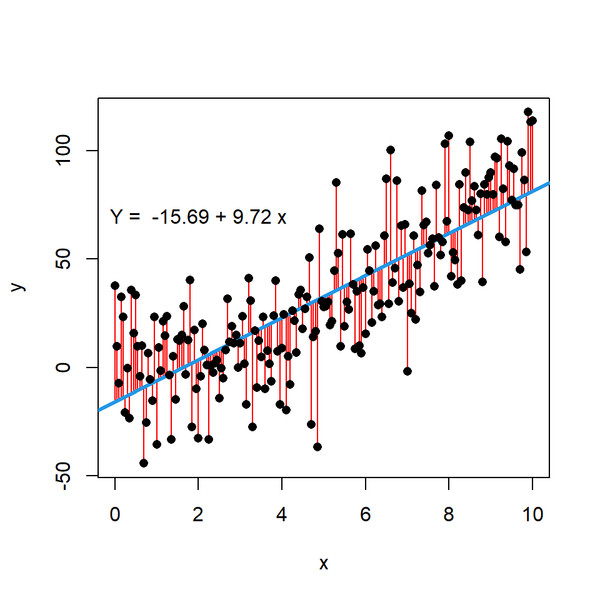
The phrase least squares means this line makes

$$\sum (y-\hat y)^2$$

as small as possible.

Why square the residuals?

• Positive and negative residuals do not cancel out
• Big misses count more than small misses

Two facts AP Stats loves:

• The LSRL always passes through $(\bar x,\bar y)$
• Regression of $y$ on $x$ is different from regression of $x$ on $y$, because the explanatory and response variables play different roles

This line is only appropriate when the scatterplot looks linear and the residual plot shows no pattern.

Finding the Regression Equation

In this course, you usually get the line from technology, not by hand from raw data. What you need is to read the output correctly.

Reading the coefficients

• In $\hat y=a+bx$, $a$ is the intercept and $b$ is the slope
• In a calculator display written as $ax+b$, $a$ is the slope and $b$ is the intercept
• A row labeled Intercept or Constant gives the intercept
• The row named for the explanatory variable gives the slope

You should also recognize:

• $r$ = correlation
• $r^2$ = coefficient of determination

Useful formulas from summary stats

If you are given $\bar x,\bar y,s_x,s_y,$ and $r$, then

$$b=r\frac{s_y}{s_x} \qquad a=\bar y-b\bar x$$

Example with $\bar x=4,\ \bar y=18,\ s_x=2,\ s_y=5,\ r=0.80$

• $b=(0.80)\left(\frac{5}{2}\right)=2$
• $a=18-(2)(4)=10$

So the line is $\hat y=10+2x$.

Built-in check. Plug in $x=\bar x=4$:

• $\hat y=10+2(4)=18=\bar y$

Also remember:

• The sign of $b$ matches the sign of $r$
• If $r=0$, then $b=0$ and the line is $\hat y=\bar y$

Interpreting the Slope and Intercept

These must be stated in context.

Slope

Template:

• For each 1-unit increase in $x$, the predicted $y$ increases/decreases by $b$ units

Example: if $x=$ hours studied and $y=$ quiz score, and $b=4.2$,

• For each additional hour studied, the predicted quiz score increases by 4.2 points.

Say predicted. That word matters. The slope describes association, not automatic causation.

Intercept

Template:

• When $x=0$, the predicted value of $y$ is $a$

Only interpret it if $x=0$ makes sense and is in a reasonable range.

Skip the interpretation when:

• $x=0$ is impossible or illogical
• $x=0$ is outside the data range, so it is extrapolation
• the predicted $y$ at 0 is impossible in context

What $r$ and $r^2$ Tell You

$r$ is the correlation coefficient. It tells you the direction and strength of the linear relationship. It has no units.

$r^2$ is the coefficient of determination. It tells you the proportion of variation in the response variable $y$ explained by its linear relationship with $x$.

Example: if $r^2=0.64$,

• About 64% of the variation in quiz scores is explained by the linear relationship between hours studied and quiz score.

If you know $r^2$ but not $r$,

• $|r|=\sqrt{r^2}$
• use the slope’s sign to choose positive or negative

Common traps:

• $r^2$ is not the percent of points on the line
• $r^2$ is not prediction accuracy
• $r^2$ does not prove causation
• high $r^2$ does not prove a linear model is appropriate

When to Use It and Common Mistakes

Use the LSRL when:

• both variables are quantitative
• the scatterplot is roughly linear
• the residual plot has no clear pattern

A curved residual plot like this one is a warning sign that a linear model is not appropriate.

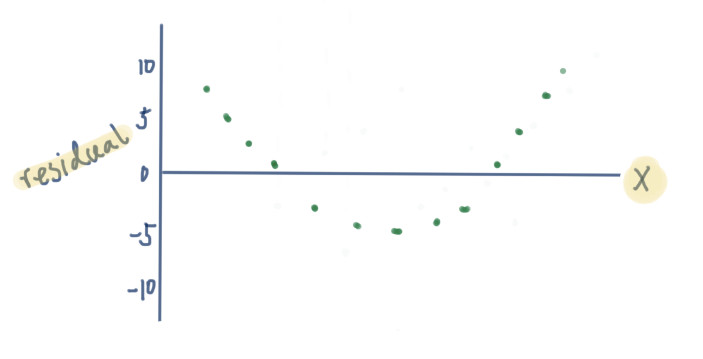
Residual plot with a curved pattern

Use it for prediction within the observed $x$-range. Outside that range, you are extrapolating, and the line may stop making sense.

Common mistakes that lose points fast:

• writing $y=a+bx$ instead of $\hat y=a+bx$
• mixing up slope and intercept from output
• saying slope is the actual change instead of the predicted change
• forcing an intercept interpretation when $x=0$ is meaningless
• saying $r^2$ explains variation in $x$ instead of $y$
• treating high $r$ or high $r^2$ as proof of causation or guaranteed strong predictions