Topic 5.4 Notes – Residuals

What Residuals Are

When you have a regression line, it predicts a response value $\hat y$ from an explanatory value $x$.

$$\hat y = a + bx$$

For one observation, the residual compares what actually happened to what the line predicted.

$$\text{residual} = y - \hat y$$

A few things matter here:

• $y$ is the observed response value from the data.
• $\hat y$ is the predicted response value from the regression line.
• A residual is the prediction error for one point.
• The subtraction order matters. It is observed minus predicted, never the other way around.
• Residuals use the same units as the response variable because you are subtracting two response values.

Geometrically, a residual is the signed vertical distance from the point to the regression line. In the figure, the top row shows scatterplots with regression lines, and the bottom row shows the matching residual plots.

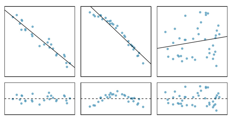
Scatterplots and their residual plots

Sign and meaning

• Positive residual means the point is above the line, so $y > \hat y$. The model underpredicted.
• Negative residual means the point is below the line, so $y < \hat y$. The model overpredicted.
• Zero residual means the point lies exactly on the line.

The size of the residual, $|\text{residual}|$, tells how far off the prediction was. The sign only tells direction.

Calculating and Interpreting a Residual

Suppose a regression line predicting quiz score from study hours is

$$\hat y = 50 + 5x$$

If a student studied $x=4$ hours and actually scored $y=73$:

1. Find the predicted value

   $$\hat y = 50 + 5(4) = 70$$

2. Compute the residual

   $$y - \hat y = 73 - 70 = 3$$

3. Interpret it in context

   The model underpredicted the student’s quiz score by 3 points.

If the observed score had been 68 instead:

$$68 - 70 = -2$$

Now the model overpredicted the student’s quiz score by 2 points.

Useful rearrangements sometimes show up:

• $y = \hat y + \text{residual}$
• $\hat y = y - \text{residual}$

Common mistakes:

• Reversing the subtraction and flipping the sign
• Saying “overpredicted by $-2$” instead of “overpredicted by 2 points”
• Rounding $\hat y$ too early

What a Residual Plot Shows

A residual plot is a scatterplot of residuals against either:

• the explanatory values $x$, or
• the predicted values $\hat y$

Each original data point becomes one point on this new graph.

• Against $x$, the plotted point is $(x, y-\hat y)$
• Against predicted value, the plotted point is $(\hat y, y-\hat y)$

The horizontal line at 0 splits positive and negative residuals. In these examples, the residuals are plotted against fitted values, which is another name for predicted values.

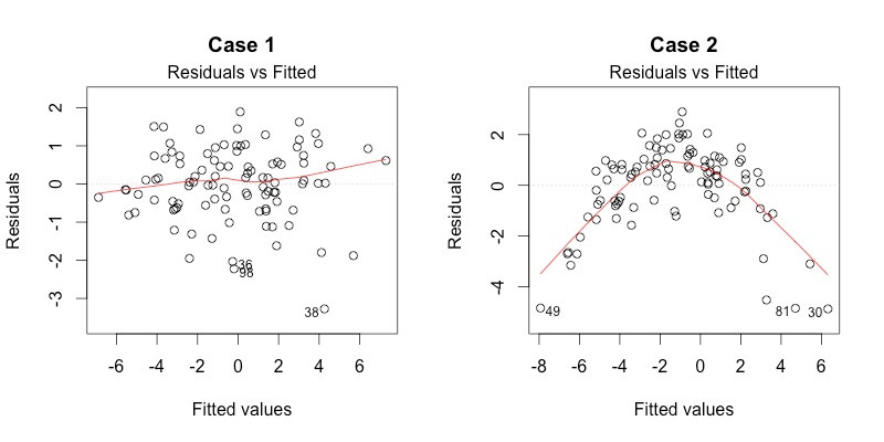
Residual plots against fitted values

This matters because the linear trend has already been removed. So the residual plot shows what pattern is still left unexplained.

• Above 0 means observed > predicted
• Below 0 means observed < predicted
• Farther from 0 means a bigger miss

Using Residual Plots to Judge a Linear Model

This is the main job of residual plots. You are checking whether a linear model is appropriate.

What you want is apparent randomness:

• points scattered above and below 0
• no clear upward or downward trend
• no curve or other pattern

Then you can say the association has a linear form, so simple linear regression is appropriate.

The three residual plots below show the key contrast. Focus on the left panel for a good linear fit, then compare it to the curved patterns in the middle and right panels.

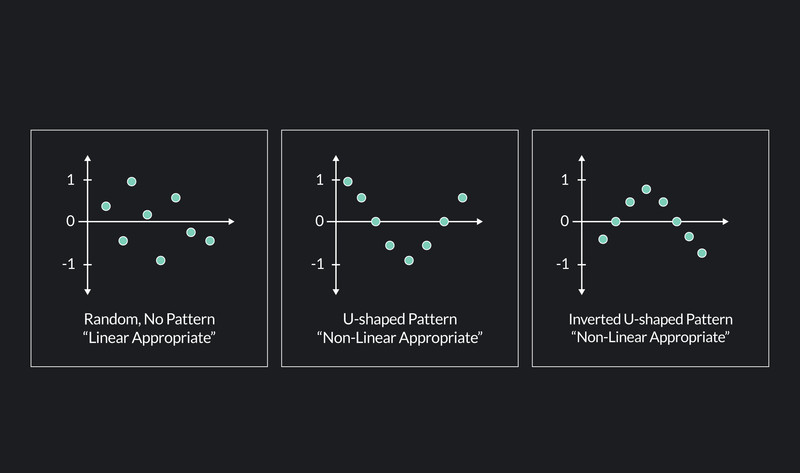
Curvature means the line missed the shape:

• U-shape
  positive residuals at low and high $x$, negative in the middle
  The line underpredicts at the ends and overpredicts in the middle.
• Upside-down U
  negative residuals at the ends, positive in the middle
  The line overpredicts at the ends and underpredicts in the middle.

Mixed positive and negative residuals by themselves are normal. The issue is whether they form a pattern.

What to Say on the Exam and Where Students Slip

Good AP-style wording sounds like this:

• “The residual plot shows apparent randomness with no clear pattern, so a linear model is appropriate.”
• “The residual plot shows a clear curved pattern, so a linear model is not appropriate.”

You need both parts:

• describe the pattern
• state what it means for the model

A few easy traps:

• A random residual plot does not mean predictions are perfect.
• Residual plots do not prove causation.
• Correlation alone does not decide whether a linear model fits. The residual plot is the check.
• One huge residual might mean one badly predicted point. It does not automatically mean nonlinearity.
• A changing spread pattern is still nonrandom, even if it is not curved.