Topic 4.1 Notes – Sampling Distributions for Sample Means

What the Sampling Distribution of x̄ Is

For one random sample of size $n$, the sample mean is

$$\bar{x}=\frac{x_1+x_2+\cdots+x_n}{n}$$

That $\bar{x}$ is just one sample’s average. If you imagined taking all possible random samples of that same size and averaging each one, the distribution of those averages is the sampling distribution of $\bar{x}$.

Three distributions show up here, and mixing them up is one of the most common mistakes:

• Population distribution
  All individual values in the population. Mean $=\mu$, standard deviation $=\sigma$.
• One sample’s data distribution
  The actual values in the sample you collected. Mean $=\bar{x}$, standard deviation $=s$.
• Sampling distribution of $\bar{x}$
  All possible sample means from repeated samples of size $n$. Mean $=\mu_{\bar{x}}$, standard deviation $=\sigma_{\bar{x}}$.

The picture below compares the population distribution with sampling distributions of $\bar{x}$ for two sample sizes. Keep your focus on the repeated-sample distributions centered at $\mu$.

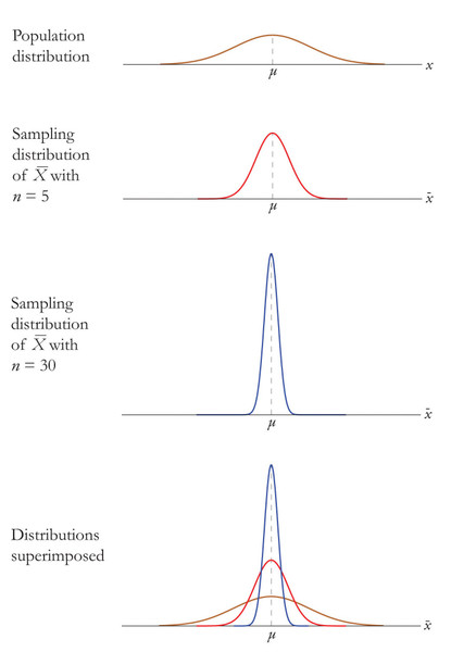
Population distribution and sampling distributions of $\bar{x}$

This is a long-run theoretical distribution. You usually do not list all possible samples. A simulation can approximate it by repeatedly sampling and recording means.

The key idea is simple. Sample means vary, but averaging several values makes them less variable than individual observations.

Center and Spread of the Sampling Distribution

The center comes first:

$$\mu_{\bar{x}}=\mu$$

That means the sample mean is an unbiased estimator of the population mean. Over many random samples of size $n$, the average of the sample means will equal the true population mean.

Be careful here. This does not mean your one sample mean must equal $\mu$.

The spread is

$$\sigma_{\bar{x}}=\frac{\sigma}{\sqrt{n}}$$

as long as the sampled values are independent.

What this means in words:

• $\sigma_{\bar{x}}$ is the typical distance of sample means from $\mu$
• it uses the same units as the original variable
• for sample-mean problems, use $\sigma/\sqrt{n}$, not $\sigma$

Larger samples keep the same center but shrink the spread. In the graph, all three sampling distributions are centered at $\mu=50$, but the curves get narrower as $n$ increases.

• Multiply $n$ by 4 $\rightarrow$ spread is cut in half
• Multiply $n$ by 9 $\rightarrow$ spread is cut by 3
• Double $n$ $\rightarrow$ spread is divided by $\sqrt{2}$

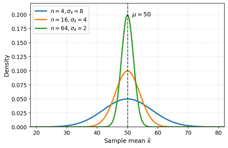
Sampling distributions of $\bar{x}$ for different sample sizes

A bigger sample improves precision. It does not fix bad sampling.

Conditions and Shape

Two separate questions matter here.

Independence

These conditions justify the formulas for center and spread:

• Randomization means the data come from a random sample or another valid random process.
• 10% condition matters when sampling without replacement from a finite population. Check $n \le 0.10N$.

If sampling is with replacement, you do not need the 10% condition.

Shape

These conditions justify using normal probability calculations:

• If the population is normal, then $\bar{x}$ is normal for any sample size.
• If the population is not normal, the Central Limit Theorem says $\bar{x}$ is approximately normal for large enough $n$.
• In AP Stats, $n \ge 30$ is the usual rule of thumb.
• If the population is extremely skewed or has extreme outliers, you may need a much larger sample.

The CLT changes the shape of the sampling distribution of means, not the population itself.

Describing and Using the Sampling Distribution

A complete description gives shape, center, and spread in context.

A standard AP-style response usually sounds like this:

1. Define the variable as $\bar{x}$, the sample mean.
2. Check randomization and the 10% condition if sampling without replacement.
3. Justify the shape using population normality or the CLT.
4. State $\mu_{\bar{x}}=\mu$.
5. State $\sigma_{\bar{x}}=\sigma/\sqrt{n}$.

For probabilities, once the sampling distribution is normal or approximately normal, use

$$z=\frac{\bar{x}-\mu}{\sigma/\sqrt{n}}$$

Example. Suppose household electricity use has $\mu=31$, $\sigma=18$, and $n=100$.

$$\mu_{\bar{x}}=31,\qquad \sigma_{\bar{x}}=\frac{18}{\sqrt{100}}=1.8$$

If you want $P(\bar{x}>34)$,

$$z=\frac{34-31}{1.8}=1.67$$

So $P(\bar{x}>34)\approx 0.048$.

In context, about 4.8% of random samples of 100 households would have a mean electricity use above 34 kilowatt-hours.

That probability is about sample means, not individual households.