Topic 3.4 Notes – Justifying a Claim Based on a Confidence Interval for a Population Proportion

What a Confidence Interval for a Population Proportion Means

A quick refresher on symbols helps everything else click. $p$ is the true population proportion, like the true proportion of all voters in a city who support a bond. $\hat p$ is the sample proportion you actually computed from sample data.

A confidence interval uses $\hat p$ to estimate $p$ with a range, because one sample does not give a perfect answer.

The correct AP Stats interpretation sounds like this:

“We are $C\%$ confident that the interval from $L$ to $U$ contains the true proportion of [population] who [characteristic].”

Your sentence must include all 4 pieces:

• confidence level
• parameter $p$, the true population proportion
• population
• success/response being measured

What “$C\%$ confident” means is long-run. If you took many random samples of the same size and built intervals the same way each time, about $C\%$ of those intervals would capture $p$.

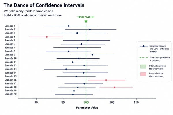
Repeated-sampling view of confidence intervals

That is exactly what the diagram is showing. Across many samples, most 95% intervals include the dashed line for the true value, and a few miss it.

One subtle point that gets tested a lot: after you calculate this interval, the interval and $p$ are both fixed. This interval either contains $p$ or it doesn’t.

So these are wrong:

• “There is a $95\%$ probability that $p$ is in this interval.”
• “$95\%$ of the population is in the interval.”
• “The sample proportion is probably correct.”

Also, your conclusion only applies to the population the sampling method supports.

Using the Interval to Judge a Claim

This is the reasoning pattern AP Stats wants to see in words.

1. Identify $p$ in context.
2. Interpret the interval in context.
3. Compare the claim value to the interval.
4. Write a cautious conclusion.

Exact-value claims

Suppose a $95\%$ CI is $(0.52, 0.62)$.

• If a claim says $p=0.60$, then 0.60 is inside the interval. It is plausible.
  • Conclusion: the interval does not provide convincing evidence that $p \ne 0.60$.
• If a claim says $p=0.50$, then 0.50 is outside the interval.
  • Conclusion: the interval provides convincing evidence that $p \ne 0.50$.
• If the claim value is exactly an endpoint, treat it as included.

Direction and threshold claims

This is where “majority” questions show up.

• Entire interval above $p_0$ → supports $p>p_0$
• Entire interval below $p_0$ → supports $p<p_0$
• Interval crosses $p_0$ → no convincing evidence for either strict direction

Example with $(0.52, 0.62)$:

• “A majority support the policy” means $p>0.50$
• Since the whole interval is above 0.50, the data support the claim

Use AP-style wording:

• provides convincing evidence
• supports the claim
• does not provide convincing evidence

Avoid words like proves, guarantees, or definitely.

What the Interval Can and Cannot Establish

Values inside the interval are plausible. They are not proven true. Values outside are not plausible at that confidence level. They are not impossible.

The interval helps you judge a claim, but it does not tell you the exact true value of $p$.

It also only reflects sampling variability. It does not fix bias from:

• undercoverage
• nonresponse
• response bias
• bad wording or flawed data collection

A narrow interval from a biased sample can still be very misleading.

Margin of Error and Interval Width

For a one-proportion $z$-interval,

$$\hat p \pm z^*\sqrt{\frac{\hat p(1-\hat p)}{n}}$$

The standard error is

$$SE_{\hat p}=\sqrt{\frac{\hat p(1-\hat p)}{n}}$$

The margin of error is

$$MOE=z^*\cdot SE_{\hat p}$$

Endpoints come from center $\pm$ margin of error. Interval width is

$$U-L=2(MOE)$$

So the margin of error is half the width. Narrower interval means a more precise estimate.

How Confidence Level and Sample Size Change the Width

Higher confidence means bigger $z^*$, bigger MOE, and a wider interval.

• 90% → $z^*=1.645$
• 95% → $z^*=1.96$
• 99% → $z^*=2.576$

The center $\hat p$ stays the same. Only the spread changes.

Larger sample size means smaller standard error, so the interval gets narrower. Width is approximately proportional to $\frac{1}{\sqrt{n}}$.

That’s why:

• doubling $n$ does not cut width in half
• cutting width in half needs about 4 times the sample size
• cutting width to one-third needs about 9 times the sample size