Topic 3.2 Notes – Sampling Distributions for Sample Proportions

What the Sampling Distribution of p̂ Is

A population proportion $p$ is the true proportion in the whole population with some trait. In AP Stats, a success just means the category you’re counting.

If a sample of size $n$ has $X$ successes, the sample proportion is

$$\hat p=\frac{X}{n}$$

So if 42 out of 100 students say they have a job, then $\hat p = 42/100 = 0.42$.

The sampling distribution of $\hat p$ is the distribution of sample proportions from many repeated random samples of the same size. That’s the part students mix up a lot. This is not the distribution of individual yes/no responses in one sample. It’s a distribution of a statistic.

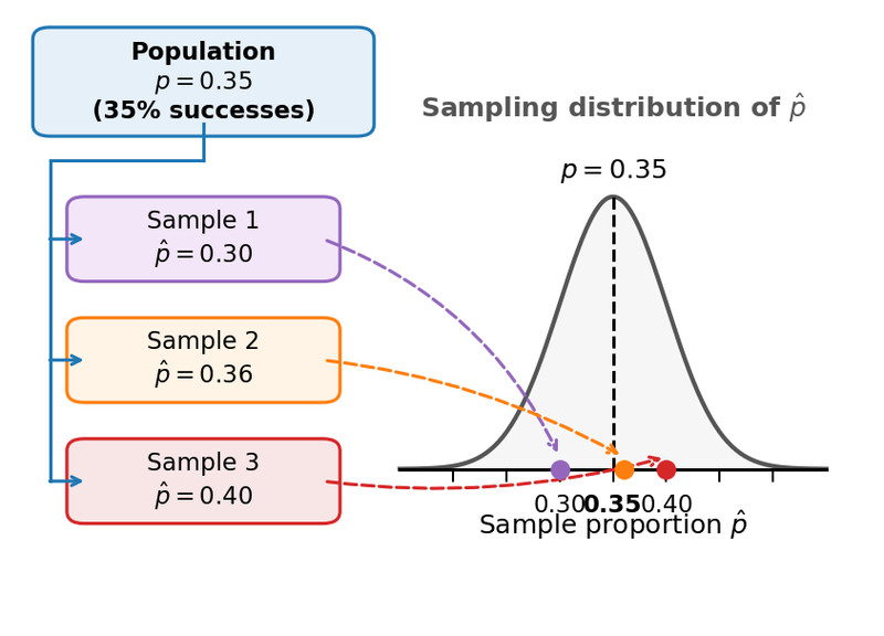
This picture shows the big idea. Start with one population that has true proportion $p = 0.35$. Different random samples from that same population give different $\hat p$ values like 0.30, 0.36, and 0.40, and those sample proportions build the sampling distribution.

If each observation is independent and has probability $p$ of success, then the number of successes follows a binomial model:

$$X \sim \text{Binomial}(n,p)$$

Since $\hat p = X/n$, the behavior of $\hat p$ comes from binomial ideas. The exact distribution of $\hat p$ is discrete because possible values go $0, \frac{1}{n}, \frac{2}{n}, \dots, 1$. Under the right conditions, though, it looks close to normal.

Center, Spread, and Shape of the Sampling Distribution

The two formulas you need are

$$\mu_{\hat p}=p$$

$$\sigma_{\hat p}=\sqrt{\frac{p(1-p)}{n}}$$

The mean says that over many random samples of size $n$, the average sample proportion will be the true proportion $p$. That’s why $\hat p$ is an unbiased estimator of $p$.

The standard deviation tells you the usual sample-to-sample change in $\hat p$. If $\sigma_{\hat p}=0.04$, then sample proportions tend to be about 0.04 away from $p$, or about 4 percentage points away.

A couple patterns matter a lot:

• Changing $p$ changes the center and the spread.
• The spread is largest when $p=0.5$, because $p(1-p)$ is biggest there.
• Increasing $n$ keeps the center the same but makes the spread smaller by the $1/\sqrt{n}$ pattern.

Shape depends on conditions. If $p$ is near 0, the distribution can be right-skewed. If $p$ is near 1, it can be left-skewed. If expected successes and failures are both large enough, it’s approximately normal.

Conditions to Use the Model

These conditions do two different jobs. One checks independence. The other checks approximate normality.

• Randomization condition
  The sample should be random, usually an SRS. A huge convenience sample still fails here.
• 10% condition
  If sampling without replacement, check $N \ge 10n$. This lets you treat observations as approximately independent. This supports the standard deviation formula.
• Large Counts condition
  Check $np \ge 10$ and $n(1-p) \ge 10$. Use $p$ here, not $\hat p$. If both pass, the sampling distribution of $\hat p$ is approximately normal.

If Large Counts fails, the mean and SD formulas can still work, but normal probability calculations are not justified.

Finding and Interpreting Probabilities with p̂

When conditions are met, model the sampling distribution as

$$\hat p \approx N\left(p,\sqrt{\frac{p(1-p)}{n}}\right)$$

Here’s the full move on a probability question:

1. Identify $p$ and $n$.
2. Check randomization, 10%, and Large Counts.
3. Compute $\mu_{\hat p}$ and $\sigma_{\hat p}$.
4. Standardize with
   $$z=\frac{\hat p-p}{\sqrt{p(1-p)/n}}$$
5. Use the standard normal table or calculator.

Example: suppose $p=0.35$ and $n=200$. Find $P(\hat p \ge 0.40)$.

$$\sigma_{\hat p}=\sqrt{\frac{(0.35)(0.65)}{200}} \approx 0.0337$$

$$z=\frac{0.40-0.35}{0.0337}\approx 1.48$$

So $P(\hat p \ge 0.40) \approx P(Z \ge 1.48) \approx 0.069$.

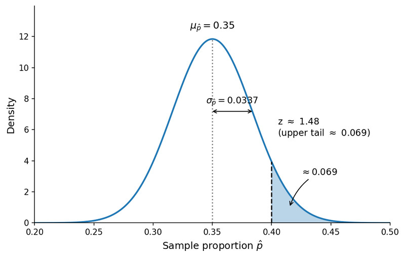
Sampling distribution of $\hat p$ with upper-tail probability

That shaded right-tail area is the probability that a random sample of 200 students has a sample proportion of at least 0.40.

In context, that means: If 35% of all students are in a club, about 6.9% of random samples of 200 students would have at least 40% in clubs.

What Students Mix Up

• Using $\hat p$ instead of $p$ in $\sigma_{\hat p}$ for this topic.
• Saying “the sample size is large” without checking $np$ and $n(1-p)$.
• Mixing up the 10% condition with Large Counts.
• Forgetting that bigger $n$ shrinks spread but does not change center.
• Treating $\sigma_{\hat p}$ as spread of individuals instead of spread of sample proportions.
• Writing probability statements about the parameter $p$ instead of about random samples and $\hat p$.