Topic 2.3 Notes – Estimating Probabilities Using Simulation

What Simulation Probability Is

A random process is repeatable chance behavior. One repetition is a trial.

From there, keep the vocabulary straight:

• An outcome is the result of one trial.
• An event is a collection of outcomes.

That sounds simple, but the meaning depends on how the trial is defined. If one trial is “one bus ride,” outcomes might be on time or late. If one trial is “the next 5 weekdays,” an outcome is a full 5-day sequence like OOTOL.

That’s why students mix up outcome and event so often. In the 5-day bus setup:

• one outcome could be OOTOO
• the event “bus is on time at least 4 of 5 days” includes many outcomes

Probability here means long-run relative frequency over many independent trials.

$$\hat P(E)=\frac{\text{\# trials where }E\text{ occurs}}{\text{\# valid trials}}$$

If an event happens in 533 out of 1000 simulated trials, then $\hat P(E)=0.533$.

One more distinction matters a lot on tests:

• Empirical probability comes from real observed data.
• Simulated probability comes from a model.

A simulation estimates the probability implied by the model. That is not automatically the same as the real-world probability.

Designing a Valid Simulation

AP readers want the full setup stated clearly. A complete simulation includes:

1. the event being estimated
2. the chance device
3. the exact assignment from random results to real outcomes
4. what counts as one full trial
5. what you record each trial
6. how many trials you repeat
7. how you compute $\hat P(E)$

Random digits

Random digits are common because each digit 0 to 9 is equally likely.

• For tenths, use single digits
  • Example: probability $0.70$ can be digits 0, 1, 2, 3, 4, 5, 6 (seven of the ten digits)
• For hundredths, use pairs 00 to 99
  • Example: probability $0.23$ can be 00 to 22

The actual labels do not matter. The proportions do.

If the outcomes do not divide evenly, extra values can be ignored.

• Simulating a fair die with digits 0 to 9
  • let 1 to 6 represent the faces
  • ignore 0, 7, 8, 9

Ignored values do not count as trials.

Independence and dependence

Complete trials should usually be independent. If the real process resets, your simulation should reset too.

Within a trial, steps may be dependent if the real process is without replacement. That difference shows up a lot in card or slip simulations.

The biggest setup mistake is defining the wrong trial. If the question asks about 5 days, one trial is the whole 5-day sequence, not one day.

How to Run and Read a Simulation

Here’s what it looks like with the bus example, where each day is on time with probability $0.70$, and the event is “at least 4 on-time days in 5 days.” Each row in the simulation output is one 5-day trial, and the highlighted rows are the successes.

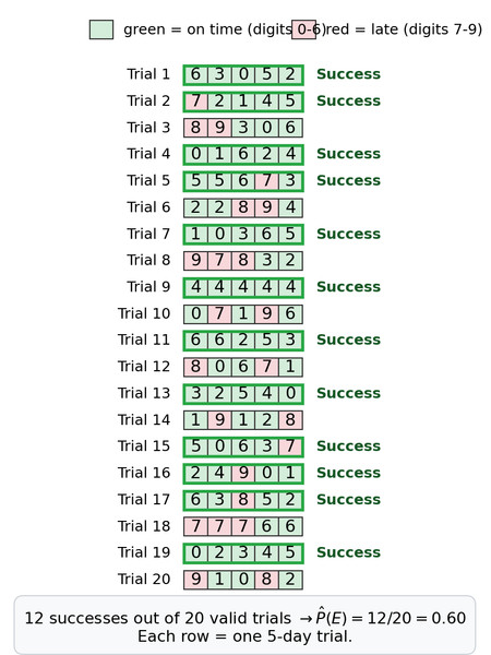
Random-digit simulation for 20 five-day bus trials

1. Generate random results from the assigned model.
2. Group them into complete trials.
3. Check whether the event happened in each trial.
4. Count successes and valid trials.
5. Compute $\hat P(E)$.
6. Interpret in context using approximately.

In the output shown, 12 out of 20 five-digit trials are successes, so $\hat P(E)=12/20=0.60$. In context, The simulation estimates that the probability the bus is on time at least 4 of the next 5 weekdays is approximately 0.60.

When reading output, count rows or completed trials, not individual digits. The denominator is valid completed trials only.

Why More Trials Help

The law of large numbers says that for independent trials, the relative frequency gets closer to the true probability as the number of trials increases. In the graph, the early estimates swing a lot, then the cumulative relative frequency settles in near the true value $p=0.53$.

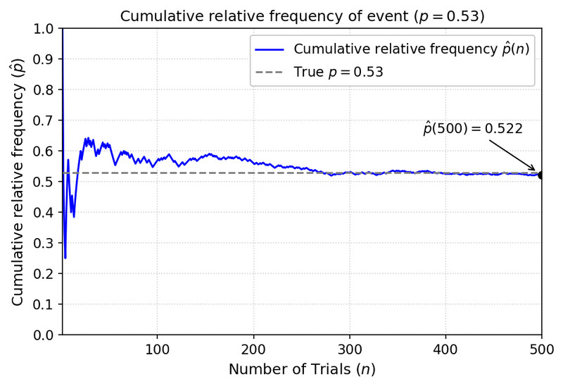
Cumulative relative frequency approaching the true probability

So in practice:

• short runs are jumpy
• long runs are more stable
• two good simulations can still give different answers
• more trials usually make those answers closer together

What this law does not say:

• the estimate improves after every single trial
• a finite simulation must match exactly
• the model itself is realistic

What Students Mix Up

• Outcome vs. event
  Outcome is one result of one trial. Event is one or more outcomes grouped together.

• One step vs. one full trial
  If the event covers several days, spins, or draws, the trial includes all of them.

• Simulated vs. true probability
  Simulation estimates the model’s probability. Real observations estimate the actual process.

• Law of large numbers vs. gambler’s fallacy
  Independent results do not make the opposite outcome “due.” Balance appears over many trials because the total grows, not because chance corrects itself.

• Counting mistakes
  Students often count digits instead of trials, include ignored values in the denominator, or forget to state the event in context.