Topic 3.9 Notes – Sampling Distributions for the Difference Between Sample Proportions

What the Sampling Distribution of p̂₁ − p̂₂ Is

This shows up when you compare two groups on one categorical outcome, usually called success.

• Group 1 has population proportion $p_1$
• Group 2 has population proportion $p_2$
• From samples, you get $$\hat p_1=\frac{x_1}{n_1} \qquad \text{and} \qquad \hat p_2=\frac{x_2}{n_2}$$ where $x$ is the number of successes and $n$ is the sample size.

The parameter is the true difference $p_1-p_2$.
The statistic is the sample difference $\hat p_1-\hat p_2$.

The sampling distribution of $\hat p_1-\hat p_2$ is the distribution of all possible values of that sample difference from many repeated independent samples, or from many repeated random assignments in an experiment.

A few details matter a lot:

• Order matters. If you define the difference as group 1 minus group 2, keep that order everywhere.
• Reversing the order changes the sign of the difference and the center.
• Reversing the order does not change the standard deviation.
• Since proportions are between 0 and 1, values of $\hat p_1-\hat p_2$ must be between $-1$ and $1$.

The graph below ties those ideas together. Switching from $\hat p_1-\hat p_2$ to $\hat p_2-\hat p_1$ flips the distribution across 0, so the center moves from positive to negative, but the spread stays the same.

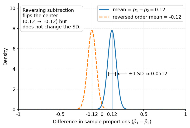
Sampling distributions for $\hat p_1-\hat p_2$ and $\hat p_2-\hat p_1$

Center, Spread, and Shape

The mean of the sampling distribution is

$$\mu_{\hat p_1-\hat p_2}=p_1-p_2$$

That means over many repeated samples, the sample difference lands at the true population difference on average. This is the unbiased idea.

The standard deviation is

$$\sigma_{\hat p_1-\hat p_2} = \sqrt{ \frac{p_1(1-p_1)}{n_1} + \frac{p_2(1-p_2)}{n_2} }$$

Why are those two parts added if the proportions are subtracted? Because the groups are independent, so the variances add.

• Do not add standard deviations.
• Add the variances inside the square root, then take the square root.
• Bigger $n_1$ or $n_2$ makes the standard deviation smaller.

The exact distribution is discrete because proportions come from counts. When counts are large enough, it is approximately normal, centered at $p_1-p_2$ with the SD above.

Conditions for Using the Normal Model

You check conditions for each group separately, not with one combined sample.

Randomization and independence

• For sampling, you need two independent random samples, one from each population.
• For experiments, you need random assignment to create independent groups.
• This does not apply to paired or matched data.

The 10% condition

This only matters for sampling without replacement from finite populations.

• Check $n_1 \leq 0.10N_1$
• Check $n_2 \leq 0.10N_2$

You do not need this for randomized experiments or sampling with replacement.

Large counts

All four expected counts must be at least 10:

• $n_1p_1 \geq 10$
• $n_1(1-p_1) \geq 10$
• $n_2p_2 \geq 10$
• $n_2(1-p_2) \geq 10$

These use population proportions $p_1$ and $p_2$, not sample proportions. If this fails, the mean and SD formulas still describe center and spread, but the normal approximation may be poor.

Finding Probabilities with p̂₁ − p̂₂

Suppose $p_1=0.42$, $p_2=0.30$, $n_1=200$, $n_2=150$, and you want $P(\hat p_1-\hat p_2 \geq 0.20)$.

1. Define the order. Here it is first group minus second group.
2. Check conditions.
   Large counts work since $200(0.42)=84$, $200(0.58)=116$, $150(0.30)=45$, $150(0.70)=105$.
3. Compute the mean.
   $$p_1-p_2=0.42-0.30=0.12$$
4. Compute the SD.
   $$\sqrt{\frac{0.42(0.58)}{200}+\frac{0.30(0.70)}{150}} \approx 0.0512$$
5. Standardize:
   $$z=\frac{d-(p_1-p_2)}{\sqrt{\frac{p_1(1-p_1)}{n_1}+\frac{p_2(1-p_2)}{n_2}}}$$ $$z=\frac{0.20-0.12}{0.0512}\approx 1.56$$
6. Use the standard normal distribution.
   $P(Z\geq 1.56)\approx 0.059$

In context, about 5.9% of repeated sample pairs would produce a sample proportion difference of at least 0.20.

Interpretation and Common Mistakes

Your interpretation always has to name both groups and keep the subtraction order.

• Mean interpretation
  Over many repeated samples, the sample proportion for group 1 minus the sample proportion for group 2 would average $p_1-p_2$.
• Standard deviation interpretation
  $\hat p_1-\hat p_2$ typically varies from the true difference $p_1-p_2$ by about the SD.
• Probability interpretation
  This is the chance of getting a certain sample difference from repeated sampling, not the chance that $p_1-p_2$ changes.

Common mistakes:

• switching from $p_1-p_2$ to $\hat p_2-\hat p_1$ halfway through
• doing one 10% check instead of one for each population
• checking only total sample size for large counts
• plugging in sample proportions when the problem gives true $p_1$ and $p_2$
• claiming one group causes a higher proportion when the data came from samples, not a randomized experiment