Topic 4.6 Notes – Approximating Values of a Function Using Local Linearity and Linearization

1. Local Linearity and the Tangent Line Approximation

If a function is differentiable at $x = a$, then very close to that point, the graph looks linear. When you zoom in enough, curves look straight. That “straight” behavior is captured by the tangent line.

You already know:

• $f(a)$ gives the point on the graph.
• $f'(a)$ gives the slope of the tangent line there.

Put those together and you get the linearization formula:

$$L(x) = f(a) + f'(a)(x - a)$$

This is just point-slope form written using function notation.

Important facts:

• $L(a) = f(a)$
• $L'(a) = f'(a)$
• $L(x) \approx f(x)$ when $x$ is close to $a$

Here’s what that looks like visually. The blue curve is $y = f(x)$ and the green line is the tangent line at the red point $(a, f(a))$.

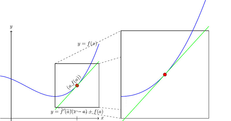
Local linearity and the tangent line approximation

In the zoomed-in view, the line and curve almost sit on top of each other near $a$, then drift apart as you move away. That “local” part is everything.

2. Constructing and Using a Linearization

When a problem asks you to approximate a value using local linearity, the steps are mechanical.

Step 1: Identify the point of tangency

You need:

• A specific $a$
• The value $f(a)$

Sometimes it’s given. Sometimes you calculate it.

Step 2: Find the slope at that point

Compute $f'(a)$.

Example:

Let $f(x) = \sqrt{x+5}$.
Approximate $f(4.1)$.

We pick $a = 4$ because that’s close and easy.

• $f(4) = \sqrt{9} = 3$
• $f'(x) = \frac{1}{2\sqrt{x+5}}$
• $f'(4) = \frac{1}{2\cdot 3} = \frac{1}{6}$

Step 3: Write the tangent line

$$L(x) = 3 + \frac{1}{6}(x - 4)$$

Step 4: Approximate the value

$$f(4.1) \approx L(4.1) = 3 + \frac{1}{6}(0.1)$$

$$= 3 + \frac{0.1}{6} = 3 + 0.0167 \approx 3.0167$$

That’s your estimate.

On a no-calculator multiple choice question, this is often faster than evaluating a messy radical directly.

3. When Linearization Is Appropriate

You should think “tangent line approximation” when:

• The input value is close to a nice number.
• The function is messy (roots, trig, exponentials).
• You are given only $f(a)$ and $f'(a)$, not the full formula.
• A differential equation gives you slope information.

If the new x-value is far from $a$, accuracy drops quickly. Local linearity only works locally.

On FRQs, they often give you a table with $f(a)$ and $f'(a)$ and expect you to build the tangent line from that data alone.

4. Underestimates and Overestimates

Whether your approximation is too big or too small depends on concavity, which comes from the second derivative.

Concave Up $(f''(a) > 0)$

• Graph bends upward.
• Tangent line lies below the curve.
• Linearization is an underestimate.

Concave Down $(f''(a) < 0)$

• Graph bends downward.
• Tangent line lies above the curve.
• Linearization is an overestimate.

The picture below shows both cases. Focus on how the tangent line sits relative to the curve near the point of tangency.

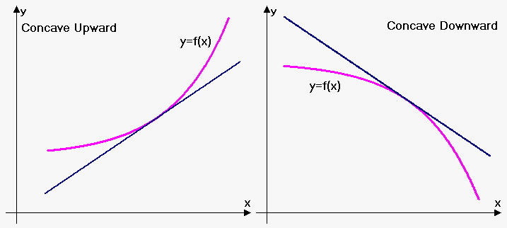
Concavity and tangent line position

On an FRQ, you must justify this using the second derivative. A complete explanation sounds like: “Since $f''(a) > 0$, the function is concave up at $a$, so the tangent line lies below the graph near $a$. Therefore, the approximation is an underestimate.”

They want the reasoning, not just the word.