Topic 7.8 Notes – Exponential Models with Differential Equations

The Exponential Differential Equation

The core model is

$$\frac{dy}{dt} = ky$$

This says: the rate of change of $y$ is proportional to $y$ itself.

Break it down:

• $y(t)$ is the amount at time $t$.
• $\frac{dy}{dt}$ is how fast it’s changing at that instant.
• $k$ is a constant of proportionality.

What $k$ tells you:

• $k > 0$ → exponential growth
• $k < 0$ → exponential decay
• Larger $|k|$ → faster change
• Units of $k$ are per unit time (like per year, per hour)

So if a population grows at a rate proportional to its size, or a chemical decays at a rate proportional to the amount present, this is the model.

Here’s what the graph behavior looks like for $k > 0$ and $k < 0$:

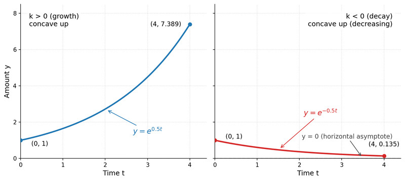
Exponential growth and decay for $\frac{dy}{dt} = ky$

Notice both are concave up. Growth increases and bends upward. Decay decreases but still curves upward toward $y = 0$.

Solving the Equation

You should immediately recognize the general solution:

$$y = Ce^{kt}$$

If you’re given an initial condition $y(0) = y_0$, then:

$$y = y_0 e^{kt}$$

Where:

• $C$ or $y_0$ is the initial amount.
• $e^{kt}$ models continuous growth or decay.

Why this works (separation of variables)

Very quickly, the reasoning:

1. Start with $\frac{dy}{dt} = ky$
2. Separate:

   $$\frac{1}{y} dy = k dt$$

3. Integrate:

   $$\ln|y| = kt + C$$

4. Exponentiate:

   $$y = Ce^{kt}$$

You rarely have to re-derive this on a quiz. You’re expected to recognize the form immediately.

Finding a Particular Model from Data

Most problems give:

• An initial value
• Another data point
• A prediction question

Example setup (new numbers):

A culture starts with 500 cells. After 4 hours, it has 800 cells.

You write:

$$y = 500e^{kt}$$

Plug in the second point:

$$800 = 500e^{4k}$$

Divide:

$$1.6 = e^{4k}$$

Take natural log:

$$\ln(1.6) = 4k$$

$$k = \frac{\ln(1.6)}{4}$$

Then substitute that $k$ back into the model.

When solving for time instead, you isolate the exponential, take natural log, and solve for $t$. Always natural log, since the model uses base $e$.

A common AP-style move is giving you a doubling time. If it doubles in $T$ time units, then:

$$e^{kT} = 2$$

That relationship lets you solve for $k$ or compare future growth.

Interpreting the Model in Context

This is where points are often earned or lost.

If a problem says:

The rate at which water leaks from a tank is proportional to the amount remaining.

That sentence translates directly to:

$$\frac{dy}{dt} = ky$$

You should be able to explain:

• $y(t)$ represents the amount of water at time $t$.
• $k$ is the constant of proportionality.
• If the tank is draining, $k < 0$.

Also understand what the equation means conceptually:

• When $y$ is large, $\frac{dy}{dt}$ is large in magnitude.
• As $y$ shrinks (in decay), the rate slows down.
• For decay, $y \to 0$ as $t \to \infty$.

This shows up on FRQs where you must interpret parameters with correct units and context. Saying “$k$ is the growth constant measured in per hours” earns credit. Leaving off units sometimes costs it.

Where This Connects

You’ve already seen differential equations in motion problems. The same idea applies there. If velocity is proportional to position, or acceleration depends on velocity, similar modeling logic appears. For AP Calculus AB, the exponential case $\frac{dy}{dt} = ky$ is the main one you’re responsible for.