Topic 1.10 Notes – The Normal Distribution

1. What a Normal Distribution Is

A normal distribution is a continuous, symmetric, mound-shaped distribution described by a smooth density curve. The total area under the curve is 1, which represents 100% of possible observations.

Here’s the general shape of a normal curve:

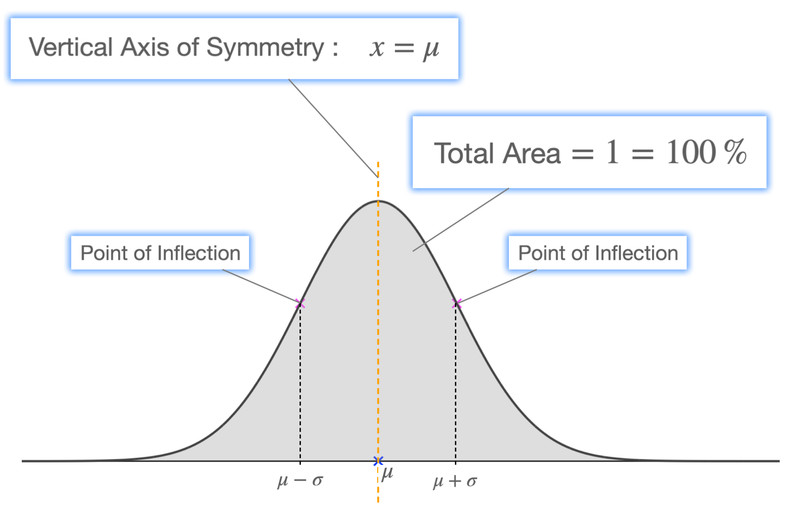
Normal distribution (bell curve) with mean μ and standard deviation σ

Key features:

• Symmetric about μ (the mean is the center and the vertical line of symmetry).
• Unimodal (one peak).
• Tails extend infinitely (they approach but never touch the axis).
• Inflection points at μ ± σ (where the curve changes concavity).

A normal distribution is completely determined by two population parameters:

• μ (mu) = population mean (center).
• σ (sigma) = population standard deviation (spread).

We write it as N(μ, σ). These are model parameters that describe a population, not sample statistics like $\bar{x}$ or $s$.

Some real-world variables are often approximately normal, like adult heights, body temperature, or the weight of loaves of bread from a well-controlled bakery. But not all data are normal.

Before using a normal model, check:

• Histogram looks roughly symmetric and unimodal.
• Normal probability plot is roughly linear.

If the data are clearly skewed or have multiple peaks, don’t force a normal model.

2. The Empirical Rule and What It Tells You

For any normal distribution, the 68-95-99.7 rule applies:

• About 68% of observations are within 1σ of μ.
• About 95% are within 2σ.
• About 99.7% are within 3σ.

The shaded regions in the normal curve below show these percentages centered at μ.

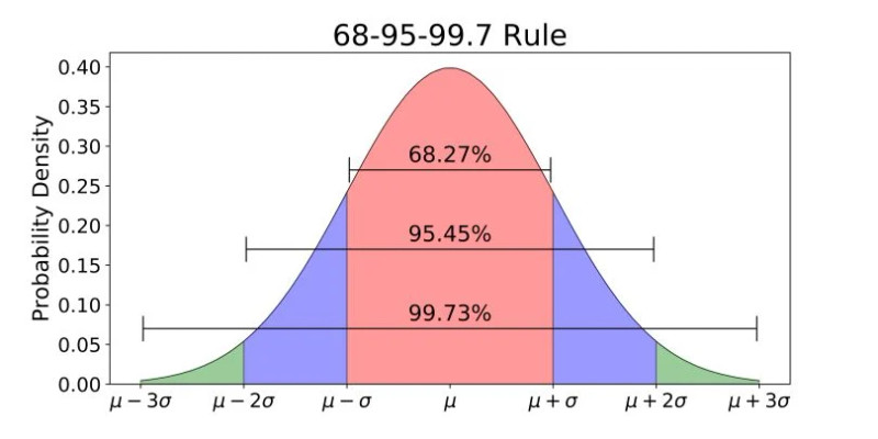
Empirical Rule for a normal distribution

This lets you make quick estimates without a calculator. For example, if loaf weights are N(500 grams, 5 grams), about 95% of loaves weigh between 490 and 510 grams.

Values beyond:

• 2σ are somewhat unusual.
• 3σ are very unusual.

Only use this rule if the distribution is normal. It does not apply to skewed data.

3. Z-Scores and Standardizing Values

A z-score tells how many standard deviations a value is from the mean.

$$z = \frac{x - \mu}{\sigma}$$

• $z > 0$ → above the mean
• $z < 0$ → below the mean
• Larger $|z|$ → more unusual

When you standardize, you convert a normal distribution into the standard normal distribution, N(0, 1).

• Mean becomes 0.
• Standard deviation becomes 1.
• Units disappear.

Example: If body temperature is N(98.6°F, 0.6°F), and someone’s temperature is 99.4°F:

$$z = \frac{99.4 - 98.6}{0.6} = \frac{4}{3} \approx 1.33$$

That temperature is about 1.33 standard deviations above average.

Transformations:

• Adding/subtracting a constant changes the mean, not shape or spread.
• Multiplying/dividing by a constant changes mean and standard deviation, not shape.

MC questions love asking what happens to mean and standard deviation after transformations.

4. Finding Proportions and Percentiles in a Normal Distribution

Once you standardize, you use technology.

A. Finding a Proportion Given a Value

Suppose bread weights are N(500, 5). What proportion weigh less than 508 grams?

1. Convert to z:
   $z = (508 - 500)/5 = 1.6$
2. Use calculator:
   normalcdf(-1E99, 508, 500, 5)
   or use standard normal with z = 1.6.
3. Interpret in context.

You would say:
“About 0.945 of loaves weigh less than 508 grams.”

Always answer in context, not just with a decimal.

Left of a value = cumulative area.
Right of a value = 1 minus left area.
Between two values = subtract cumulative areas.

B. Finding a Value Given a Percentile

Suppose the bakery wants the top 10% heaviest loaves.

1. Area to the left is 0.90.
2. Use invNorm(0.90, 500, 5).
3. Interpret.

You might get about 506.4 grams.

So the cutoff for the heaviest 10% is about 506.4 grams.

This shows up when you’re asked for minimum qualifying scores or percentiles.

5. Comparing Relative Position with Z-Scores and Percentiles

Two ways to describe relative standing:

• Z-score → number of standard deviations from the mean.
• Percentile → percent of observations at or below a value.

If you’re comparing scores from different tests with different spreads, raw scores are meaningless. Compare z-scores instead.

Higher z-score = better relative performance.

Percentiles are easier to explain in context.
Z-scores are better for mathematical comparison.

On FRQs, if you’re asked who performed better relative to their group, compute and compare z-scores.