Topic 6.2 Notes – Constructing a Confidence Interval for a Population Proportion

1. The One-Sample z-Interval for a Population Proportion

You use this procedure when:

• You have one sample
• The variable is categorical (yes/no, success/failure)
• You want to estimate a single population proportion $p$

The sample gives you a sample proportion:

$$\hat{p} = \frac{x}{n}$$

where $x$ is the number of “successes” and $n$ is the sample size.

Every confidence interval has this structure:

$$\text{point estimate} \pm \text{margin of error}$$

For a proportion:

• Point estimate → $\hat{p}$
• Standard error →
  $$SE_{\hat{p}} = \sqrt{\frac{\hat{p}(1-\hat{p})}{n}}$$
• Margin of error →
  $$ME = z^* \sqrt{\frac{\hat{p}(1-\hat{p})}{n}}$$

So the full interval is:

$$\hat{p} \pm z^* \sqrt{\frac{\hat{p}(1-\hat{p})}{n}}$$

$z^*$ comes from the standard normal distribution and depends on confidence level:

• 90% → 1.645
• 95% → 1.96
• 99% → 2.576

On the AP exam, this formula is not printed for you, but you can build it from “statistic ± (critical value)(standard error)” and the standard error formula.

2. Conditions for Inference

No conditions, no inference credit. Even if your math is perfect.

Random

Data must come from a random sample or randomized experiment.
If the sample wasn’t random, you cannot generalize to the population.

Independence

When sampling without replacement, check:

$$\frac{n}{N} \le 0.10$$

In words: the population is at least 10 times the sample size.
State it in context, not just as a formula.

Large Counts Condition

We need the sampling distribution of $\hat{p}$ to be approximately normal.

Check:

$$n\hat{p} \ge 10 \quad \text{and} \quad n(1-\hat{p}) \ge 10$$

That means at least 10 expected successes and 10 expected failures.

Important detail: for confidence intervals, use $\hat{p}$ in this check. (Using a hypothesized $p$ is for hypothesis tests, which is next topic.)

3. How to Construct the Interval

Here’s how it flows on a quiz or FRQ.

1. State the parameter and procedure
   “We want to estimate $p$, the true proportion of ___ in the population. A one-sample z-interval for a proportion is appropriate.”
2. Check conditions
   Random, 10%, Large Counts - all in context.
3. Calculate
   • Find $\hat{p} = x/n$
   • Find $z^*$
   • Compute standard error
   • Compute margin of error
   • Write the interval
4. Interpret in context

Correct model:

We are 95% confident that the true proportion of [population + variable] is between ___ and ___.

You must mention:

• Confidence level
• Population
• Variable
• The word “proportion”

Do not say there is a 95% chance the true proportion is in this interval.

To picture where $z^*$ comes from, think about the middle area of the normal curve. The critical value cuts off the middle chunk that matches your confidence level.

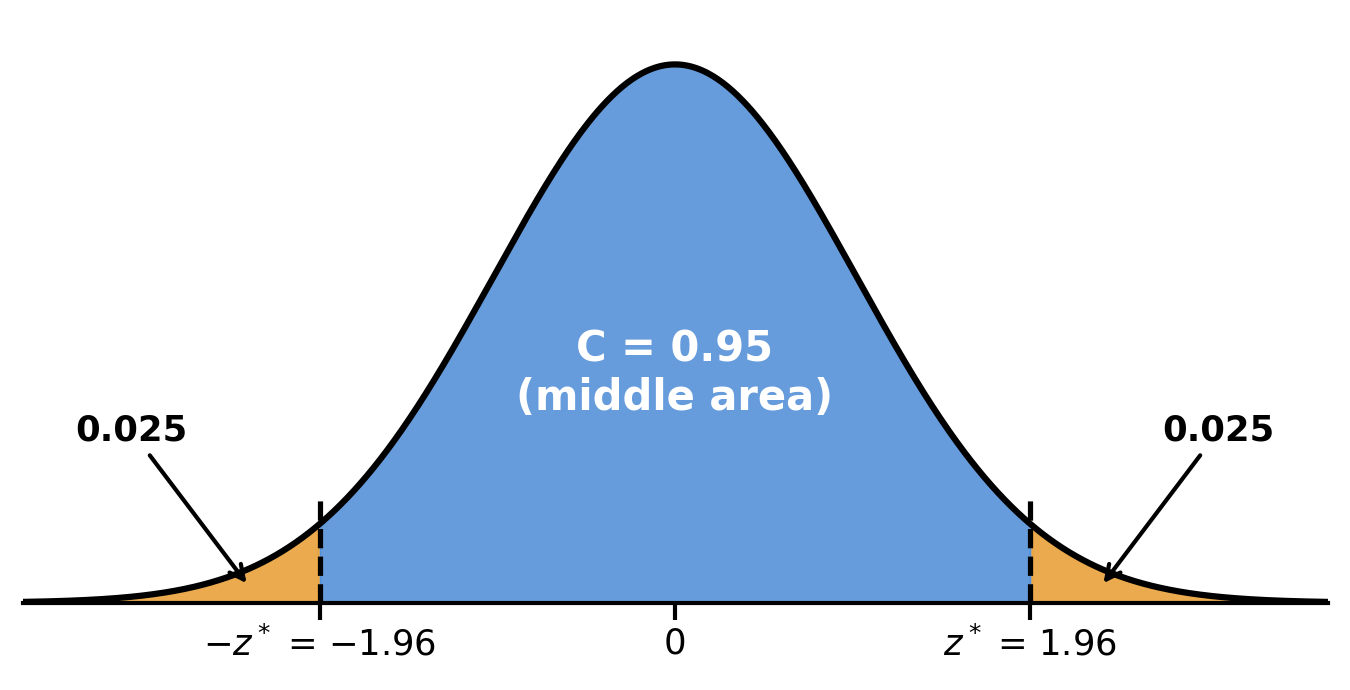
For 95% confidence, the middle area $C = 0.95$ lies between $-z^* = -1.96$ and $z^* = 1.96$, leaving 0.025 in each tail.

The shaded middle area represents the confidence level. For a 95% confidence interval, you want the central 0.95 of the distribution, which gives $z^* \approx 1.96$.

Calculator shortcut (TI-84):
STAT → TESTS → 1-PropZInt → enter $x$, $n$, confidence level.

4. Margin of Error and Sample Size

The margin of error is:

$$ME = z^* \sqrt{\frac{\hat{p}(1-\hat{p})}{n}}$$

Three big ideas:

• Higher confidence → larger $z^*$ → wider interval
• Larger $n$ → smaller standard error → narrower interval
• Variability is largest when $\hat{p} = 0.5$

Finding Required Sample Size

Rearranging gives:

$$n = \left(\frac{z^*}{ME}\right)^2 p(1-p)$$

To plan ahead:

• Use a previous estimate for $p$, or
• Use $p = 0.5$ for the most conservative (largest) sample size.

Always round up. If you round down, your margin of error might be too large.

5. What Confidence Level Means

The correct meaning:

If we repeated this sampling method many times, about C% of the resulting intervals would capture the true population proportion.

The parameter $p$ is fixed. The interval changes from sample to sample.

That subtle wording difference shows up constantly in AP grading.