Topic 6.1 Notes – Introducing Statistics: Why Be Normal?

Random vs Non‑Random Variation in Distribution Shapes

When you take multiple random samples from the same population, their graphs will not look identical. That’s normal. The shape, center, and spread will wiggle around a bit.

The real question is why they look different.

Random variation

This is the natural fluctuation you expect from sample to sample.

• Caused purely by chance.
• Happens even with perfect random sampling.
• No consistent pattern across repeated samples.
• Differences are usually small and centered around the same general value.

For example, imagine repeatedly sampling 50 voters from the same city. The sample proportions who support a candidate might be 0.48, 0.52, 0.50, 0.46. The histograms won’t be identical, but they’ll look similar overall.

Non‑random variation

This shows up when something systematic is happening.

Possible causes:

• Biased sampling (undercoverage, convenience sampling)
• Measurement problems
• Confounding variables
• Actual subgroups in the population

These often produce patterns like:

• Consistently shifted centers
• Strong skewness
• Bimodal distributions (suggesting two groups)

The big idea from this topic: Variation might be random, or it might signal something real. Because we can’t be certain, all statistical conclusions involve uncertainty.

That uncertainty is exactly why we need probability models.

What Questions Should You Ask When Shapes Differ?

If two samples from the same population look different, pause and think.

• Is the difference in center larger than what chance alone would produce?
• Is one distribution much more spread out than expected?
• Did the sampling method introduce bias?
• If we repeated this many times, would this result be common?

On quizzes and FRQs, you may be shown two dotplots or histograms from samples and asked what the variation suggests. The strongest answers mention random sampling variability unless there’s clear evidence of a systematic issue.

This leads directly to sampling distributions.

Sampling Distributions and Being “Normal”

A sampling distribution is the distribution of a statistic (like $\hat{p}$) from many repeated random samples of the same size.

Important distinction:

• The data distribution = distribution of individual observations.
• The sampling distribution = distribution of a statistic across samples.

When we do inference for proportions, we rely on the sampling distribution of $\hat{p}$.

When conditions are met, that sampling distribution is approximately normal. For example, the graph below shows the sampling distribution of $\hat{p}$ centered at the true proportion $p = 0.35$, with standard deviation $\sqrt{\frac{p(1-p)}{n}}$. The shaded region represents a probability such as $P(0.33 < \hat{p} < 0.37)$.

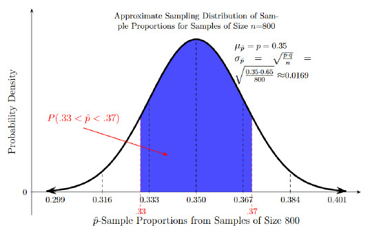
When this distribution is approximately normal, we can:

• Use z-scores
• Calculate probabilities
• Build confidence intervals
• Conduct hypothesis tests

If it’s not approximately normal, those z-based methods are not valid.

Notice this does not require the raw data to be normal. It’s the sampling distribution of the statistic that needs to be approximately normal.

The Large Counts Condition for Proportions

To justify a normal approximation for $\hat{p}$, we check the Large Counts Condition:

$$np \ge 10 \quad \text{and} \quad n(1-p) \ge 10$$

These represent:

• Expected successes ≥ 10
• Expected failures ≥ 10

If both are satisfied, the sampling distribution of $\hat{p}$ is approximately normal.

Quick example

Suppose a manufacturer claims 30% of customers prefer a new flavor. You take a random sample of $n = 80$.

Check:

• $np = 80(0.30) = 24$
• $n(1-p) = 80(0.70) = 56$

Both are ≥ 10, so the sampling distribution of $\hat{p}$ is approximately normal.

On tests, you must actually show these calculations. Writing “Large Counts satisfied” without numbers won’t earn credit.

Also watch this detail:

• For hypothesis tests, use the claimed population proportion $p$.
• For confidence intervals, use the sample proportion $\hat{p}$.

Students mix that up constantly.

Why This Matters for Inference

All of Unit 6 depends on this logic:

1. Samples vary because of random variation.
2. We model that variation with a sampling distribution.
3. If that sampling distribution is approximately normal, we can calculate how unusual a result is.
4. That helps us decide whether what we observed is likely just chance.

Inference is basically asking, “Is this difference bigger than random variation would typically produce?”

Normality lets us answer that with math instead of guessing.